Bioinformatic analysis

1. Setting up the R environment

Before beginning our bioinformatic analysis, we need to prepare the R environment by setting the working directory and loading the required R packages. While base R provides essential functions, many specialised tools, like those for processing metabarcoding data, are developed by the community and distributed as packages. These packages are collections of functions, documentation, and datasets published by researchers to address specific analytical needs. For example, we’ll use packages like dada2 for quality filtering and denoising during the bioinformatic pipeline. Installing and loading these packages extends R’s capabilities, leveraging open-source collaboration to make cutting-edge methods accessible. This modularity is one of R’s greatest strengths, enabling reproducible and efficient workflows.

Let’s open a new R script, save it as bioinformatic_pipeline.R in the bootcamp folder, set the current working directory to the bootcamp folder, and, finally, load all necessary packages we will be using during the bioinformatic analysis.

## set up the working environment
setwd(file.path(Sys.getenv("HOME"), "Desktop", "bootcamp"))
# package ShortRead needs to be installed, but not loaded
required_packages <- c("dada2", "ggplot2", "gridExtra", "readr",
  "ggpubr", "stringr", "tidyverse", "scales")
for (pkg in required_packages) {
  if (!require(pkg, character.only = TRUE)) {
    stop(paste("Package", pkg, "is not installed. Please install it before proceeding."))
  } else {
    message(pkg, " version: ", packageVersion(pkg))
  }
}

Output

Loading required package: dada2
Loading required package: Rcpp
dada2 version: 1.28.0
Loading required package: ggplot2
ggplot2 version: 3.5.1
Loading required package: gridExtra
gridExtra version: 2.3
Loading required package: dplyr

Attaching package: ‘dplyr’

The following object is masked from ‘package:gridExtra’:

    combine

The following objects are masked from ‘package:stats’:

    filter, lag

The following objects are masked from ‘package:base’:

    intersect, setdiff, setequal, union

dplyr version: 1.1.4
Loading required package: readr
readr version: 2.1.5
Loading required package: ggpubr
ggpubr version: 0.6.0
Loading required package: stringr
stringr version: 1.5.1
Loading required package: tidyverse
── Attaching core tidyverse packages ────────────────────────────────────────────────────────────── tidyverse 2.0.0 ──
✔ forcats   1.0.0     ✔ tibble    3.2.1
✔ lubridate 1.9.3     ✔ tidyr     1.3.1
✔ purrr     1.0.2     
── Conflicts ──────────────────────────────────────────────────────────────────────────────── tidyverse_conflicts() ──
✖ dplyr::combine() masks gridExtra::combine()
✖ dplyr::filter()  masks stats::filter()
✖ dplyr::lag()     masks stats::lag()
ℹ Use the conflicted package to force all conflicts to become errors
tidyverse version: 2.0.0
Loading required package: scales

Attaching package: ‘scales’

The following object is masked from ‘package:purrr’:

    discard

The following object is masked from ‘package:readr’:

    col_factor

scales version: 1.3.0

A bit more information about the code block above (as it might look a bit daunting at first):

1. #: We can use this symbol to “comment out” code lines. This method is frequently used to provide more information about the code.

2. required_packages: is a character vector containing all the package names we want to load.

3. for(): is a function loop, iterating over each element of required_packages.

4. !require(): tries to load a package (library), but if not successfully loaded, it will prompt you to install this package.

5. message(): prints a formatted message for each package.

Understanding loops for efficient coding

Writing loops, such as the for() loop above, are very common in bioinformatic pipelines, as they avoid repetitive code writing. For example, the for() loop above can also be written as (without the necessary check for the need to install a package first):

library(dada2); packageVersion("dada2")
library(ggplot2); packageVersion("ggplot2")
library(gridExtra); packageVersion("gridExtra")
library(dplyr); packageVersion("dplyr")
library(readr); packageVersion("readr")
library(ggpubr); packageVersion("ggpubr")
library(stringr); packageVersion("stringr")
library(tidyverse); packageVersion("tidyverse")
library(scales); packageVersion("scales")

Loops require a bit of practise to understand and write, as they contain very specific syntax. We recommend practicing often to get the hang of it :)

Now that we have created a variable (required_packages), we can see this appear in the Environment window in the top-right of RStudio.

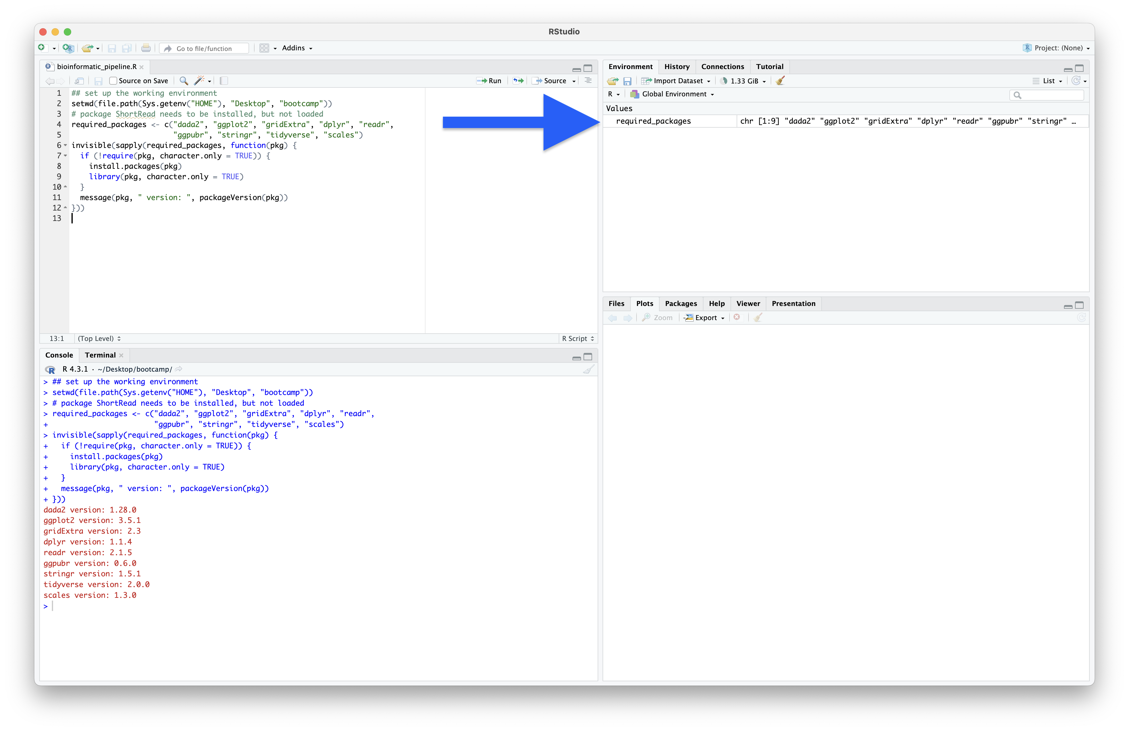
Fig. 12 : Our first variable in the Environment window

R help documentation

Consulting the R help documentation will help with understanding all aspects of the function. The help documentation for specific functions can be called using the following code:

?sapply()

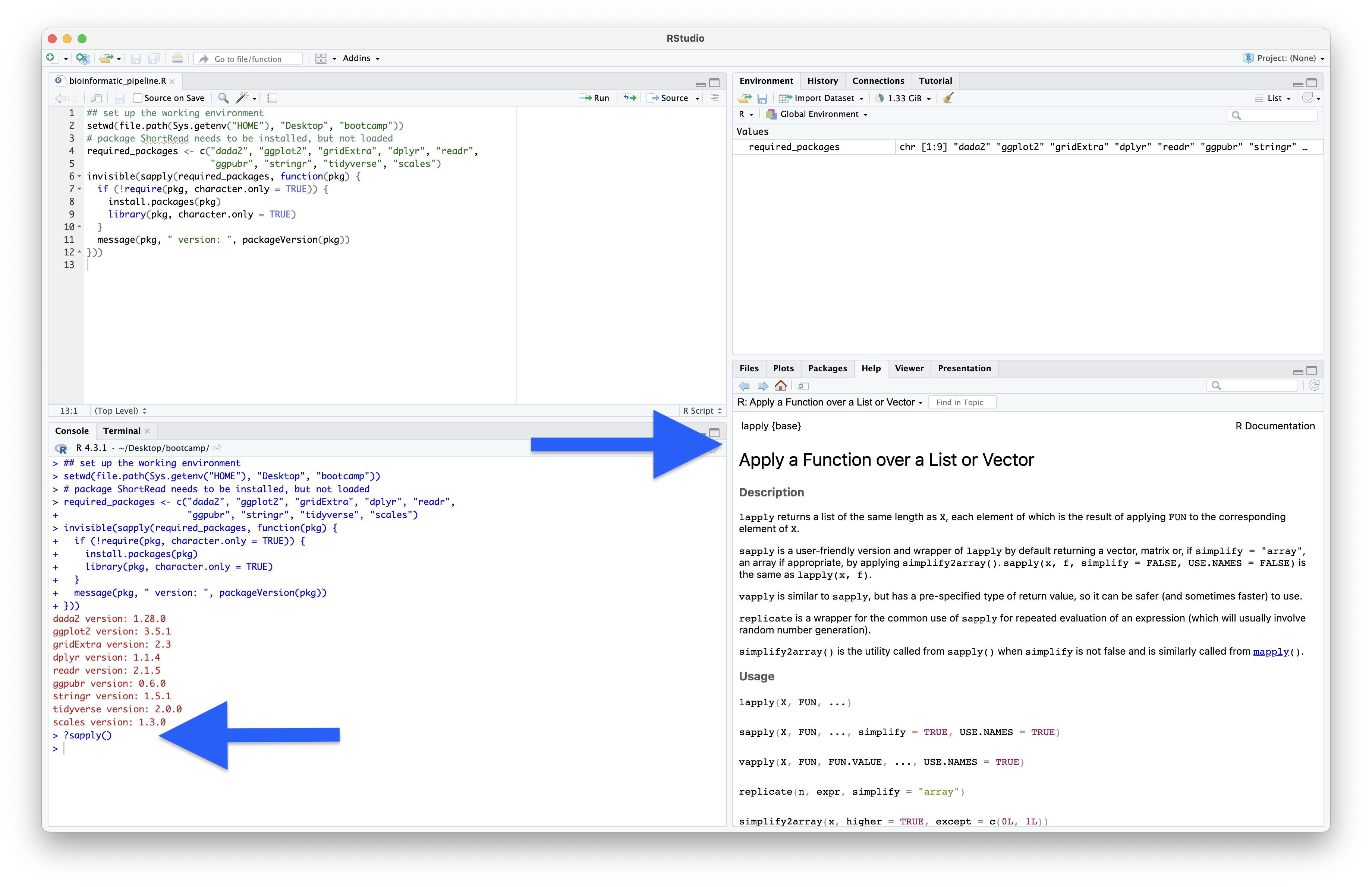
Fig. 13 : Bringing up the R help documentation using the ?function() command

2. Exploring the starting files

2.1 Sample metadata file

Now that we have set the correct working directory and loaded all necessary packages, we can read in some of the starting files and explore their contents. We will start with the metadata file. Note that the code below reads in the metadata file and pipes (%>%) the file into a new function (arrange()) to sort the table based on the sampleID column.

## Read metadata file into memory
metadata <- read_tsv(file.path("0.metadata", "sample_metadata.txt")) %>%
  arrange(sampleID)

Output

Rows: 45 Columns: 8                                                                                                 
── Column specification ──────────────────────────────────────────────────────────────────────────────────────────────
Delimiter: "\t"
chr (5): sampleID, collectionDate, region, sampleType, sampleLocation
dbl (3): latitude, longitude, replicate

ℹ Use `spec()` to retrieve the full column specification for this data.
ℹ Specify the column types or set `show_col_types = FALSE` to quiet this message.

The output shows that the metadata table consists of 45 rows and 8 columns. The output also lists the column headers and type of data contained within each column. We can view the metadata dataframe as a spreadsheet in the Source Editor window by clicking on the name of the variable in the Environment window.

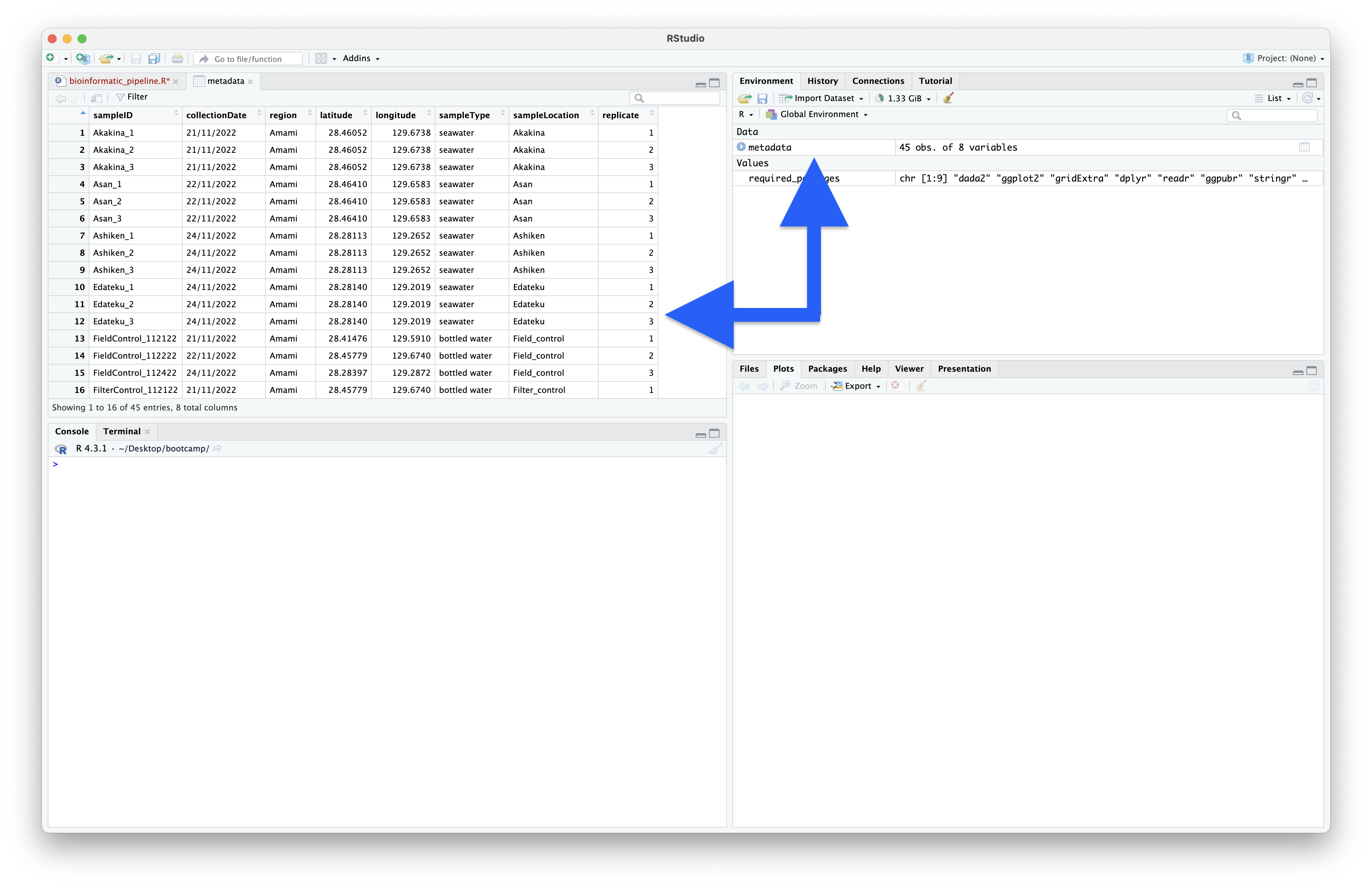
Fig. 14 : Viewing dataframes as spreadsheets in the Source Editor window by clicking on the name in the Environment window

Now, let’s look at the naming structure of the sample ID’s, as well as the different locations at which the samples were collected. We can select a specific column from an R dataframe by using the $ symbol. Furthermore, we can use indexing [] to specify the number of items. So, let’s print out the first 10 sample ID’s.

## Explore and organise data
# Print sample and file names to Console
writeLines(metadata$sampleID[1:10])

Output

> writeLines(metadata$sampleID[1:10])
Akakina_1
Akakina_2
Akakina_3
Asan_1
Asan_2
Asan_3
Ashiken_1
Ashiken_2
Ashiken_3
Edateku_1

From the output, we can see that our sample ID’s are structured as Location + _ + replicate number. It also seems that we have 3 replicates per location, which is a standard replication approach for eDNA metabarcoding surveys.

Finally, let’s print out the location ID’s within metadata. Since we have 3 replicates, it will be best to only print the unique names (function: unique()), and not repeat each location 3 times.

writeLines(unique(metadata$sampleLocation))

Output

> writeLines(unique(metadata$sampleLocation))
Akakina
Asan
Ashiken
Edateku
Field_control
Filter_control
Gamo
Heda
Imaizaki
Kurasaki
Sakibaru
Sani
Taen
Tatsugo
Yadon

The output shows that we have 15 unique location names, including 2 different control samples (Field_control and Filter_control). Multiplying 15 (number of locations) times 3 (number of replicates per location) gives us 45 samples, which is the same number as the rows in our metadata file.

2.2 Sequence files

2.2.1 Data format

Besides the metadata file, we also have access to our raw sequence files. These are stored in the 1.raw subdirectory. Since we have 45 samples, let’s count the number of raw sequence files we have.

length(list.files(path = "1.raw", pattern = "001.fastq.gz", full.names = TRUE))

Output

> length(list.files(path = "1.raw", pattern = "001.fastq.gz", full.names = TRUE))
[1] 90

We seem to have 90 files, double the number of samples. This tells us two things:

1. Samples are most likely already demultiplexed, i.e., reads have been assigned to their respective samples.

2. Samples are most likely sequenced using a paired-end Illumina sequencing strategy.

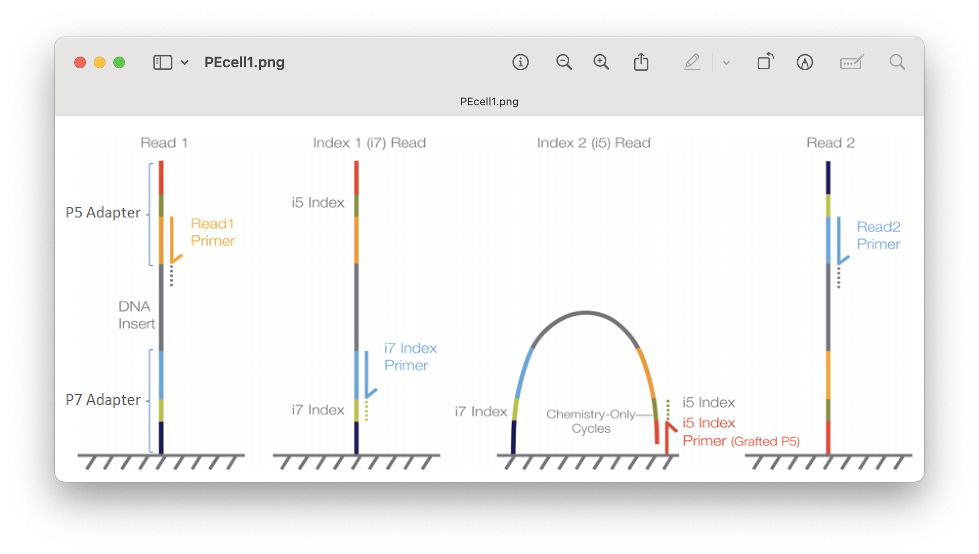
Fig. 15 : Illustration of Illumina paired-end sequencing

Let’s verify this by printing the first 10 filenames.

writeLines(list.files(path = "1.raw", pattern = "001.fastq.gz", full.names = TRUE)[1:10])

Output

> writeLines(list.files(path = "1.raw", pattern = "001.fastq.gz", full.names = TRUE)[1:10])
1.raw/Akakina_1_S103_R1_001.fastq.gz
1.raw/Akakina_1_S103_R2_001.fastq.gz
1.raw/Akakina_2_S104_R1_001.fastq.gz
1.raw/Akakina_2_S104_R2_001.fastq.gz
1.raw/Akakina_3_S105_R1_001.fastq.gz
1.raw/Akakina_3_S105_R2_001.fastq.gz
1.raw/Asan_1_S108_R1_001.fastq.gz
1.raw/Asan_1_S108_R2_001.fastq.gz
1.raw/Asan_2_S109_R1_001.fastq.gz
1.raw/Asan_2_S109_R2_001.fastq.gz

Indeed, we seem to have two files, an R1 (forward) and R2 (reverse) file, for each sample, Akakina_1, Akakina_2, Akakina_3, etc.

Data formats

The file structure observed for this data is the most common format for metabarcoding data. However, please note that your data format might deviate from this standard and will be dependent on your laboratory protocols and sequencing specifications. Other formats that are frequently observed are:

1. Demultiplexed single end: rather than paired-end, the library was sequenced single end. For this format, you will end up with a single file (`R1`) per sample, rather than two. The bioinformatic pipeline can be followed with minor modifications for this type of data, e.g., merging forward and reverse reads can be omitted.
2. Combined paired end: For this format, you will receive a single forward (`R1`) and reverse (`R2`) file for your full library. This format is usually observed when the library was constructed without following Illumina specifications. You will need to conduct demultiplexing prior to following this bioinformatic pipeline.
3. Combined single end: For this format, you will receive a single forward (`R1`) file for your full library. Besides the need to conduct demultiplexing prior to following this bioinformatic pipeline, minor modifications to the pipeline are necessary, e.g., omit the merging of forward and reverse reads step.

More recently, scientists have been exploring third-generation sequencing approaches (e.g., Oxford Nanopore Technologies) for eDNA and metabarcoding purposes. This type of data, however, requires a completely different bioinformatic pipeline for analysis. Please come have a chat with me after class if you would like some help with this type of sequencing data.

2.2.2 Renaming files

During our bioinformatic pipeline, we will use sample ID’s to identify and process sequencing files. For ease-of-use, it would be best if our sequence filenames consist only out of sample IDs plus a suffix that is shared between all forward and all reverse files (don’t worry if this sounds abstract at the moment, it will become clear once we start processing the files). However, our sequence filenames include a unique identifier in between the sample ID and common suffix. When we inspect the previous output, we can see that for sample ID Akakina_1, for example, the unique identifier is _S103, while the unique identifier is _S104 for Akakina_2. To make our lives a bit easier when processing the files, let’s remove this unique identifier now. We can print the first 10 files again to verify our code worked as expected.

# Rename sequence files for consistency
file.rename(list.files(path = "1.raw", pattern = "_001.fastq.gz", full.names = TRUE), 
            gsub("_[A-Z]\\d{2,3}", "", list.files(path = "1.raw", pattern = "_001.fastq.gz", full.names = TRUE)))
# print the first 10 sequence filenames
writeLines(list.files(path = "1.raw", pattern = "001.fastq.gz", full.names = TRUE)[1:10])

Output

> writeLines(list.files(path = "1.raw", pattern = "001.fastq.gz", full.names = TRUE)[1:10])
1.raw/Akakina_1_R1_001.fastq.gz
1.raw/Akakina_1_R2_001.fastq.gz
1.raw/Akakina_2_R1_001.fastq.gz
1.raw/Akakina_2_R2_001.fastq.gz
1.raw/Akakina_3_R1_001.fastq.gz
1.raw/Akakina_3_R2_001.fastq.gz
1.raw/Asan_1_R1_001.fastq.gz
1.raw/Asan_1_R2_001.fastq.gz
1.raw/Asan_2_R1_001.fastq.gz
1.raw/Asan_2_R2_001.fastq.gz

Looking at the output, we can see that our sequence filenames now only contain the sample ID, followed by either _R1_001.fastq.gz for the forward or _R2_001.fastq.gz for the reverse sequence file. We can, also, check if the sample IDs and sequence filenames match using the setdiff() function, i.e., ensure all sample IDs have sequence files and no sequence files exist for which no sample ID metadata is provided.

# Determine if sample and file names match
setdiff(metadata$sampleID, str_extract(list.files(path = "1.raw", pattern = "R1_001.fastq.gz"), "^[A-za-z_]+_[0-9]+"))
setdiff(str_extract(list.files(path = "1.raw", pattern = "R1_001.fastq.gz"), "^[A-za-z_]+_[0-9]+"), metadata$sampleID)

Output

> setdiff(metadata$sampleID, str_extract(list.files(path = "1.raw", pattern = "R1_001.fastq.gz"), "^[A-za-z_]+_[0-9]+"))
character(0)
> setdiff(str_extract(list.files(path = "1.raw", pattern = "R1_001.fastq.gz"), "^[A-za-z_]+_[0-9]+"), metadata$sampleID)
character(0)

3. Initial data checks

When receiving your sequencing files, it is always best to check the data prior to processing to ensure everything is as you expect or within the parameters of your chosen sequencing specifications.

3.1 Raw data quality scores

One aspect to check is if the raw data quality scores conform to Illumina standards. We can use the plotQualityProfile() function within dada2 to explore the quality scores.

## Step one: check raw sequence files
# Set variables
raw_forward_reads <- sort(list.files("1.raw", pattern = "R1_001.fastq.gz", full.names = TRUE))
raw_reverse_reads <- sort(list.files("1.raw", pattern = "R2_001.fastq.gz", full.names = TRUE))
# Determine raw quality scores
forward_raw_qual_plot <- plotQualityProfile(raw_forward_reads, aggregate = TRUE) + ggplot2::labs(title = "Forward Raw Reads") + ggplot2::theme(plot.title = ggplot2::element_text(hjust = 0.5))
reverse_raw_qual_plot <- plotQualityProfile(raw_reverse_reads, aggregate = TRUE) + ggplot2::labs(title = "Reverse Raw Reads") + ggplot2::theme(plot.title = ggplot2::element_text(hjust = 0.5))
raw_qual_plots <- ggarrange(forward_raw_qual_plot, reverse_raw_qual_plot, ncol = 2)
ggsave(filename = file.path("0.metadata", "raw_read_quality_plot_aggregated.pdf"), plot = raw_qual_plots, width = 10, height = 6)

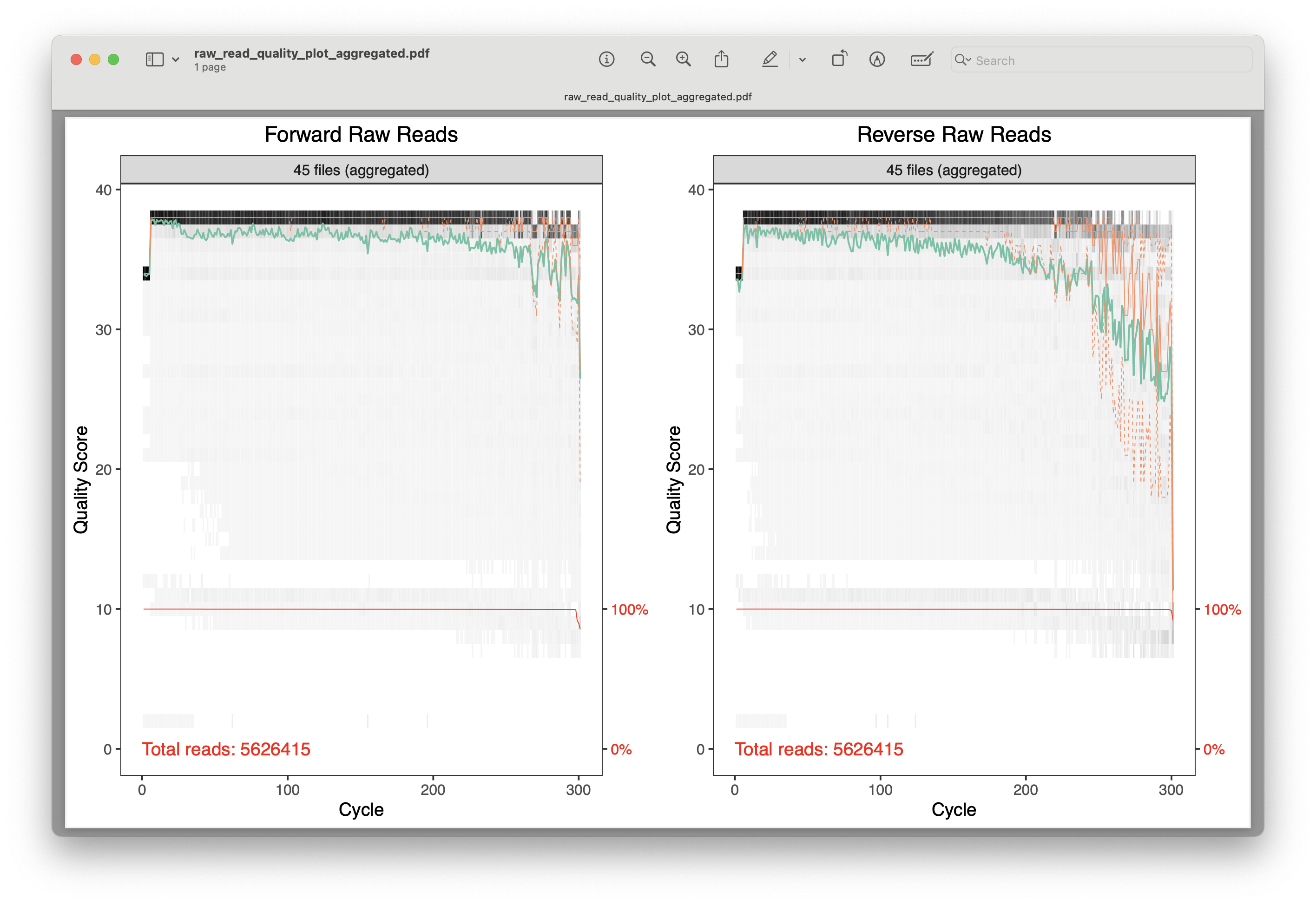
Fig. 16 : A plot of the combined raw quality scores of all forward and reverse sequence files (note the standard Illumina pattern of reduced quality at the end of the reads)

For these plots, the cycle number (or read length) is on the x-axis, while the quality score is on the y-axis. The black heatmap shows the frequency of each score at a specific base position. The green line is the mean quality score at a specific base position, while the orange line is the median, and the dashed orange lines depict the quartiles. The red line at the bottom shows the percentage of reads with this length.

For our data, the plots show that we have a total number of 5,626,415 reads for the forward and reverse sequence files, nearly all reads obtaining a length of 300 basepairs (which should match the cycle number of the kit you purchased), and an overall high quality score that conforms to the standard Illumina pattern. The number of total reads does not conform to the Illumina specifications of a V3 2x300 bp Illumina MiSeq kit. However, as this data is a subset of the sequencing run, we do not need to be alarmed.

3.2 Read count per sample

Besides investigating the quality scores, total read count, and read length, it is also useful to investigate read count per sample and determine if the forward and reverse sequencing files contain the same number of reads. Determining read count per sample can help identify low read count samples or an uneven distribution of reads across samples, which might indicate the need for resequencing some samples. Determining identical read count for forward and reverse sequencing files could help determine issues during file transfer and data integrity issues.

We will make use of our metadata file and the fact that our sequence filenames contain sample ID information. This link will help us store the read count per sample in new columns in metadata, enabling us to visualise results using the ggplot2 R package.

# Determine raw read count per sample
metadata <- metadata %>%
  mutate(
    # Forward reads
    raw_reads_f = ShortRead::countFastq(
      file.path("1.raw", paste0(sampleID, "_R1_001.fastq.gz"))
    )$records,
    # Reverse reads
    raw_reads_r = ShortRead::countFastq(
      file.path("1.raw", paste0(sampleID, "_R2_001.fastq.gz"))
    )$records
  )

# Check if forward and reverse have the same number of reads
for (i in 1:nrow(metadata)) {
  if (metadata$raw_reads_f[i] != metadata$raw_reads_r[i]) {
    cat("\nERROR: Mismatch in", metadata$sampleID[i], 
        "- F:", metadata$raw_reads_f[i], 
        "R:", metadata$raw_reads_r[i])
  }
}

# Plot raw read count per sample
mean_reads <- metadata %>%
  group_by(sampleType) %>%
  summarise(mean_reads = mean(raw_reads_f))
type_colors <- scales::hue_pal()(length(unique(metadata$sampleType)))
names(type_colors) <- unique(metadata$sampleType)
ggplot(metadata, aes(x = reorder(sampleID, raw_reads_f), y = raw_reads_f, fill = sampleType)) +
  geom_bar(stat = "identity") +
  geom_hline(data = mean_reads, aes(yintercept = mean_reads, color = sampleType),
    linetype = "dashed", linewidth = 1, show.legend = FALSE) +
  geom_text(data = mean_reads, aes(x = -Inf, y = mean_reads + max(metadata$raw_reads_f) * 0.02,
      label = paste("Mean:", comma(round(mean_reads))),color = sampleType),
    hjust = -0.1, vjust = -0.5, size = 3, show.legend = FALSE) +
  scale_fill_manual(values = type_colors) +
  scale_color_manual(values = type_colors) +
  scale_y_continuous(labels = comma, expand = expansion(mult = c(0.05, 0.15))) +
  labs(x = "Sample ID (ordered by read count)", y = "Raw Read Count") +
  theme_minimal() +
  theme(axis.text.x = element_text(angle = 45, hjust = 1), plot.margin = margin(r = 40), legend.position = "top")
ggsave(filename = file.path("0.metadata", "per_sample_raw_read_count.png"), plot = last_plot(), bg = "white", dpi = 300)

# Calculate total read count across all samples
sum(metadata$raw_reads_f)
sum(metadata$raw_reads_r)

Output

> sum(metadata$raw_reads_f)
[1] 5626415
> sum(metadata$raw_reads_r)
[1] 5626415

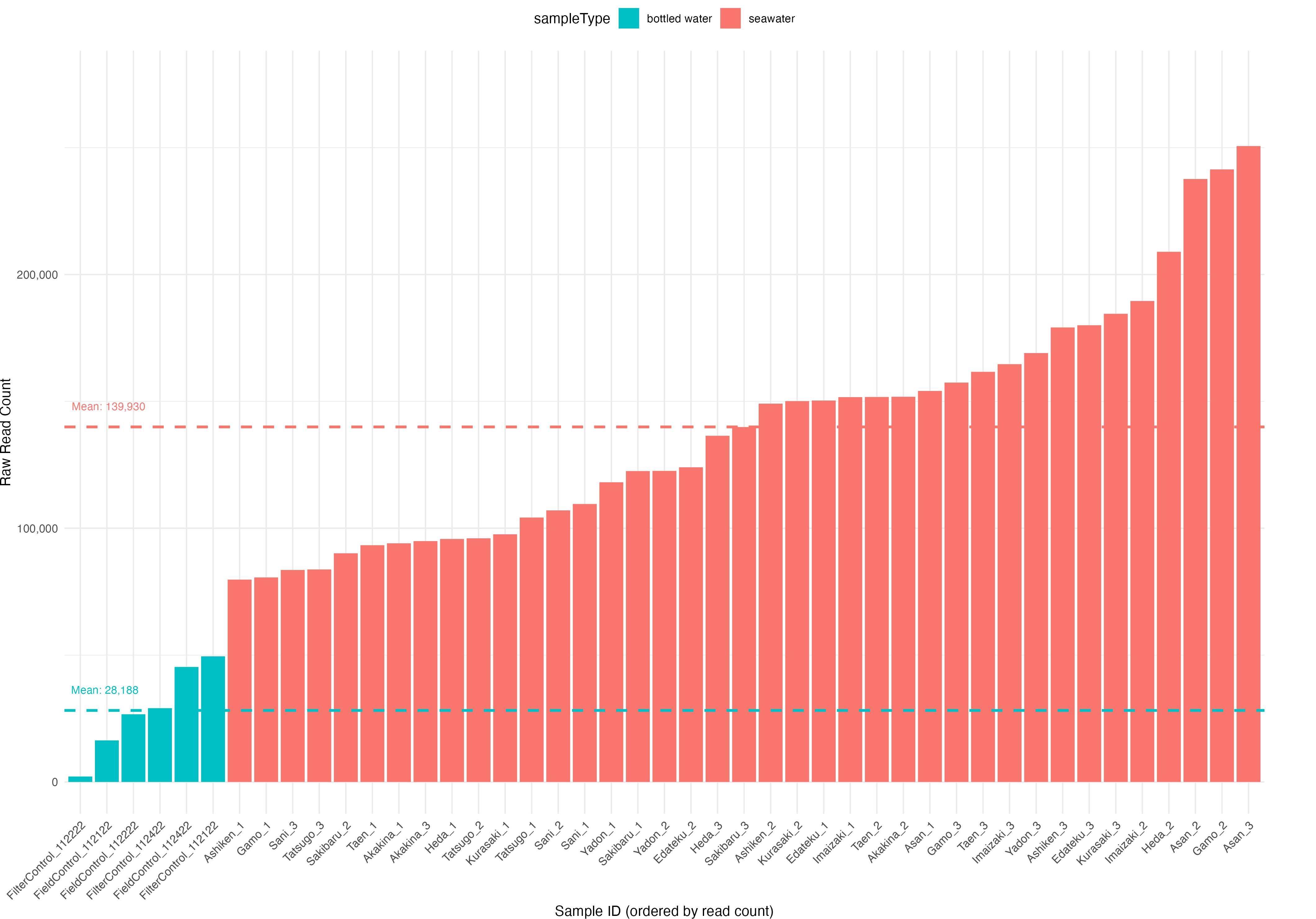
Fig. 17 : A plot showing the per sample read count, filled based on sample type

4. Removing primer sequences

While our data has been demultiplexed, i.e., barcodes removed and reads assigned to sample IDs, our data still contains the primer sequences. Since these regions are artefacts from the PCR amplification and not biological, they will need to be removed from the reads before continuing with the bioinformatic pipeline. For this library and experiment, we have used the mlCOIintF/jgHCO2198 primer set (Leray et al., 2013). The forward primer corresponds to 5’-GGWACWGGWTGAACWGTWTAYCCYCC-3’ and the reverse primer sequence is 5’-TAIACYTCIGGRTGICCRAARAAYCA-3’. Before batch processing every sample, let’s test our code on a single sample to start with. For primer or adapter removal, we can use the prgram cutadapt. Cutadapt, unfortunately, is not an R package, but rather a CLI program written in Python. Normally, this means that we have to run cutadapt through the Terminal window. However, we can make use of the system2() function in R, which allows us to run shell commands like cutadapt in an R environment.

Before running cutadapt on a single sample, let’s specify the necessary variables, including where R can find the software program (Sys.which()), the primer sequences in a cutadapt format (note that we need to specify the R2 primers in the opposite direction as the R1 primers), and a list of forward and reverse output files.

## Step two: trim primer sequences
# Set variables
cutadapt <- Sys.which("cutadapt")
system2(cutadapt, args = "--version")
if(!dir.exists("2.trimmed")) dir.create("2.trimmed")
FWD <- "GGWACWGGWTGAACWGTWTAYCCYCC"
REV <- "TANACYTCNGGRTGNCCRAARAAYCA"
FWD_RC <- rc(FWD)
REV_RC <- rc(REV)
R1_primers <- paste0("-g ", FWD, " -a ", REV_RC)
R2_primers <- paste0("-G ", REV, " -A ", FWD_RC)
trimmed_forward_reads <- file.path("2.trimmed", basename(raw_forward_reads))
trimmed_reverse_reads <- file.path("2.trimmed", basename(raw_reverse_reads))

Output

> system2(cutadapt, args = "--version")
5.0

4.1 A single sample example

Now that we have all necessary variables loaded, we can test our cutadapt code on a single sample. When using the system2() function, we specify the program, followed by a list of parameters (args = c()). For cutadapt, we need to specify which primers to remove. To only keep reds for which both primers were found and removed, we need to specify the --discard-untrimmed option. The --no-indels and -e 2 parameters allow us to tell cutadapt to not include insertions and deletions in the search and allow a maximum of 2 errors in the primer sequence. We can specify the --revcomp parameter to search for the primer sequences in both directions, while --overlap 15 requires at least a 15 basepair length match with the primer sequence. Finally, we can use the --cores=0 parameter to automatically detect the number of available cores.

system2(cutadapt, args = c(R1_primers, R2_primers, "--discard-untrimmed", 
                           "--overlap 15", "--no-indels", "-e 2", "--cores=0", 
                           "-o", trimmed_forward_reads[1], "-p", trimmed_reverse_reads[1], 
                           raw_forward_reads[1], raw_reverse_reads[1]))

Output

> system2(cutadapt, args = c(R1_primers, R2_primers, "--discard-untrimmed", 
+                            "--overlap 15", "--no-indels", "-e 2", "--cores=0", 
+                            "-o", trimmed_forward_reads[1], "-p", trimmed_reverse_reads[1], 
+                            raw_forward_reads[1], raw_reverse_reads[1]))
This is cutadapt 5.0 with Python 3.11.4
Command line parameters: -g GGWACWGGWTGAACWGTWTAYCCYCC -a TGRTTYTTYGGNCAYCCNGARGTNTA -G TANACYTCNGGRTGNCCRAARAAYCA -A GGRGGRTAWACWGTTCAWCCWGTWCC --discard-untrimmed --overlap 15 --no-indels -e 2 --cores=0 -o 2.trimmed/Akakina_1_R1_001.fastq.gz -p 2.trimmed/Akakina_1_R2_001.fastq.gz 1.raw/Akakina_1_R1_001.fastq.gz 1.raw/Akakina_1_R2_001.fastq.gz
Processing paired-end reads on 14 cores ...

=== Summary ===

Total read pairs processed:             94,059
  Read 1 with adapter:                  89,697 (95.4%)
  Read 2 with adapter:                  86,851 (92.3%)

== Read fate breakdown ==
Pairs discarded as untrimmed:           11,235 (11.9%)
Pairs written (passing filters):        82,824 (88.1%)

Total basepairs processed:    56,591,056 bp
  Read 1:    28,287,800 bp
  Read 2:    28,303,256 bp
Total written (filtered):     45,532,657 bp (80.5%)
  Read 1:    22,758,418 bp
  Read 2:    22,774,239 bp

=== First read: Adapter 1 ===

Sequence: GGWACWGGWTGAACWGTWTAYCCYCC; Type: regular 5'; Length: 26; Trimmed: 89689 times

Minimum overlap: 15
No. of allowed errors:
1-12 bp: 0; 13-25 bp: 1; 26 bp: 2

Overview of removed sequences
length	count	expect	max.err	error counts
15	4	0.0	1	2 2
16	3	0.0	1	3
17	10	0.0	1	1 9
19	39	0.0	1	28 11
20	10	0.0	1	4 6
21	42	0.0	1	23 19
22	48	0.0	1	33 15
23	44	0.0	1	17 27
24	136	0.0	1	69 67
25	1590	0.0	1	767 823
26	87619	0.0	2	62938 23850 831
27	140	0.0	2	52 57 31
28	1	0.0	2	0 0 1
30	1	0.0	2	0 0 1
33	1	0.0	2	0 1
34	1	0.0	2	0 1


=== First read: Adapter 2 ===

Sequence: TGRTTYTTYGGNCAYCCNGARGTNTA; Type: regular 3'; Length: 26; Trimmed: 8 times

Minimum overlap: 15
No. of allowed errors:
1-10 bp: 0; 11-22 bp: 1; 23 bp: 2

Bases preceding removed adapters:
  A: 0.0%
  C: 37.5%
  G: 12.5%
  T: 50.0%
  none/other: 0.0%

Overview of removed sequences
length	count	expect	max.err	error counts
26	8	0.0	2	6 2


=== Second read: Adapter 3 ===

Sequence: TANACYTCNGGRTGNCCRAARAAYCA; Type: regular 5'; Length: 26; Trimmed: 86836 times

Minimum overlap: 15
No. of allowed errors:
1-10 bp: 0; 11-22 bp: 1; 23 bp: 2

Overview of removed sequences
length	count	expect	max.err	error counts
18	1	0.0	1	0 1
19	1	0.0	1	0 1
20	1	0.0	1	1
21	10	0.0	1	8 2
22	5	0.0	1	3 2
23	29	0.0	2	25 4
24	81	0.0	2	52 29
25	1137	0.0	2	397 740
26	85503	0.0	2	83445 1575 483
27	67	0.0	2	28 12 27
170	1	0.0	2	1


=== Second read: Adapter 4 ===

Sequence: GGRGGRTAWACWGTTCAWCCWGTWCC; Type: regular 3'; Length: 26; Trimmed: 15 times

Minimum overlap: 15
No. of allowed errors:
1-12 bp: 0; 13-25 bp: 1; 26 bp: 2

Bases preceding removed adapters:
  A: 13.3%
  C: 26.7%
  G: 26.7%
  T: 33.3%
  none/other: 0.0%

Overview of removed sequences
length	count	expect	max.err	error counts
15	3	0.0	1	2 1
19	1	0.0	1	1
26	9	0.0	2	5 4
47	1	0.0	2	1
103	1	0.0	2	0 0 1

The cutadapt output provides information on how many reads were analysed, how many reads were trimmed, plus a detailed overview of where the primers were cut in the sequence. For our sample Akakina_1, 94,059 reads were processed and 82,824 (88.1%) reads were found to contain the primer sequences. As the options we specified in our command managed to remove the primer sequences from nearly all reads, we will use these settings to process all samples.

Checking results

We strongly suggest to frequently check results and confirm the expected output, especially when you are trying new code or testing parameters. In this case, for example, we can look at the number of raw reads for sample Akakina_1 that we have stored in our metadata file (metadata$raw_reads_f[1]) and see that this number matches the cutadapt report.

Optimising parameters

While the correct parameters are provided during this workshop for this data set, we suggest you spend quite a bit of time to test different parameter settings for your own data, ensuring optimal results.

4.2 Batch trimming

To batch process our cutadapt command and trim primers for all samples, we can use a for loop combined with vector indexing. Before executing the for loop with the cutadapt command, we can run through the loop and print out all the sample and file names, ensuring we point to the correct files at each stage.

for (i in seq_along(raw_forward_reads)) {
    cat("Sample ID:", metadata$sampleID[i], "\nForward In:", raw_forward_reads[i], "\nReverse In:", raw_reverse_reads[i], 
      "\nForward Out:", trimmed_forward_reads[i], "\nReverse Out:", trimmed_reverse_reads[i], "\n\n")
}

Output

> for (i in seq_along(raw_forward_reads)) {
+   cat("Sample ID:", metadata$sampleID[i], "\nForward In:", raw_forward_reads[i], "\nReverse In:", raw_reverse_reads[i], 
+       "\nForward Out:", trimmed_forward_reads[i], "\nReverse Out:", trimmed_reverse_reads[i], "\n\n")
+ }
Sample ID: Akakina_1 
Forward In: 1.raw/Akakina_1_R1_001.fastq.gz 
Reverse In: 1.raw/Akakina_1_R2_001.fastq.gz 
Forward Out: 2.trimmed/Akakina_1_R1_001.fastq.gz 
Reverse Out: 2.trimmed/Akakina_1_R2_001.fastq.gz 

Sample ID: Akakina_2 
Forward In: 1.raw/Akakina_2_R1_001.fastq.gz 
Reverse In: 1.raw/Akakina_2_R2_001.fastq.gz 
Forward Out: 2.trimmed/Akakina_2_R1_001.fastq.gz 
Reverse Out: 2.trimmed/Akakina_2_R2_001.fastq.gz 

Sample ID: Akakina_3 
Forward In: 1.raw/Akakina_3_R1_001.fastq.gz 
Reverse In: 1.raw/Akakina_3_R2_001.fastq.gz 
Forward Out: 2.trimmed/Akakina_3_R1_001.fastq.gz 
Reverse Out: 2.trimmed/Akakina_3_R2_001.fastq.gz 

Sample ID: Asan_1 
Forward In: 1.raw/Asan_1_R1_001.fastq.gz 
Reverse In: 1.raw/Asan_1_R2_001.fastq.gz 
Forward Out: 2.trimmed/Asan_1_R1_001.fastq.gz 
Reverse Out: 2.trimmed/Asan_1_R2_001.fastq.gz 

Sample ID: Asan_2 
Forward In: 1.raw/Asan_2_R1_001.fastq.gz 
Reverse In: 1.raw/Asan_2_R2_001.fastq.gz 
Forward Out: 2.trimmed/Asan_2_R1_001.fastq.gz 
Reverse Out: 2.trimmed/Asan_2_R2_001.fastq.gz 

Sample ID: Asan_3 
Forward In: 1.raw/Asan_3_R1_001.fastq.gz 
Reverse In: 1.raw/Asan_3_R2_001.fastq.gz 
Forward Out: 2.trimmed/Asan_3_R1_001.fastq.gz 
Reverse Out: 2.trimmed/Asan_3_R2_001.fastq.gz 

Sample ID: Ashiken_1 
Forward In: 1.raw/Ashiken_1_R1_001.fastq.gz 
Reverse In: 1.raw/Ashiken_1_R2_001.fastq.gz 
Forward Out: 2.trimmed/Ashiken_1_R1_001.fastq.gz 
Reverse Out: 2.trimmed/Ashiken_1_R2_001.fastq.gz 

Sample ID: Ashiken_2 
Forward In: 1.raw/Ashiken_2_R1_001.fastq.gz 
Reverse In: 1.raw/Ashiken_2_R2_001.fastq.gz 
Forward Out: 2.trimmed/Ashiken_2_R1_001.fastq.gz 
Reverse Out: 2.trimmed/Ashiken_2_R2_001.fastq.gz 

Sample ID: Ashiken_3 
Forward In: 1.raw/Ashiken_3_R1_001.fastq.gz 
Reverse In: 1.raw/Ashiken_3_R2_001.fastq.gz 
Forward Out: 2.trimmed/Ashiken_3_R1_001.fastq.gz 
Reverse Out: 2.trimmed/Ashiken_3_R2_001.fastq.gz 

Sample ID: Edateku_1 
Forward In: 1.raw/Edateku_1_R1_001.fastq.gz 
Reverse In: 1.raw/Edateku_1_R2_001.fastq.gz 
Forward Out: 2.trimmed/Edateku_1_R1_001.fastq.gz 
Reverse Out: 2.trimmed/Edateku_1_R2_001.fastq.gz 

Sample ID: Edateku_2 
Forward In: 1.raw/Edateku_2_R1_001.fastq.gz 
Reverse In: 1.raw/Edateku_2_R2_001.fastq.gz 
Forward Out: 2.trimmed/Edateku_2_R1_001.fastq.gz 
Reverse Out: 2.trimmed/Edateku_2_R2_001.fastq.gz 

Sample ID: Edateku_3 
Forward In: 1.raw/Edateku_3_R1_001.fastq.gz 
Reverse In: 1.raw/Edateku_3_R2_001.fastq.gz 
Forward Out: 2.trimmed/Edateku_3_R1_001.fastq.gz 
Reverse Out: 2.trimmed/Edateku_3_R2_001.fastq.gz 

Sample ID: FieldControl_112122 
Forward In: 1.raw/FieldControl_112122_R1_001.fastq.gz 
Reverse In: 1.raw/FieldControl_112122_R2_001.fastq.gz 
Forward Out: 2.trimmed/FieldControl_112122_R1_001.fastq.gz 
Reverse Out: 2.trimmed/FieldControl_112122_R2_001.fastq.gz 

Sample ID: FieldControl_112222 
Forward In: 1.raw/FieldControl_112222_R1_001.fastq.gz 
Reverse In: 1.raw/FieldControl_112222_R2_001.fastq.gz 
Forward Out: 2.trimmed/FieldControl_112222_R1_001.fastq.gz 
Reverse Out: 2.trimmed/FieldControl_112222_R2_001.fastq.gz 

Sample ID: FieldControl_112422 
Forward In: 1.raw/FieldControl_112422_R1_001.fastq.gz 
Reverse In: 1.raw/FieldControl_112422_R2_001.fastq.gz 
Forward Out: 2.trimmed/FieldControl_112422_R1_001.fastq.gz 
Reverse Out: 2.trimmed/FieldControl_112422_R2_001.fastq.gz 

Sample ID: FilterControl_112122 
Forward In: 1.raw/FilterControl_112122_R1_001.fastq.gz 
Reverse In: 1.raw/FilterControl_112122_R2_001.fastq.gz 
Forward Out: 2.trimmed/FilterControl_112122_R1_001.fastq.gz 
Reverse Out: 2.trimmed/FilterControl_112122_R2_001.fastq.gz 

Sample ID: FilterControl_112222 
Forward In: 1.raw/FilterControl_112222_R1_001.fastq.gz 
Reverse In: 1.raw/FilterControl_112222_R2_001.fastq.gz 
Forward Out: 2.trimmed/FilterControl_112222_R1_001.fastq.gz 
Reverse Out: 2.trimmed/FilterControl_112222_R2_001.fastq.gz 

Sample ID: FilterControl_112422 
Forward In: 1.raw/FilterControl_112422_R1_001.fastq.gz 
Reverse In: 1.raw/FilterControl_112422_R2_001.fastq.gz 
Forward Out: 2.trimmed/FilterControl_112422_R1_001.fastq.gz 
Reverse Out: 2.trimmed/FilterControl_112422_R2_001.fastq.gz 

Sample ID: Gamo_1 
Forward In: 1.raw/Gamo_1_R1_001.fastq.gz 
Reverse In: 1.raw/Gamo_1_R2_001.fastq.gz 
Forward Out: 2.trimmed/Gamo_1_R1_001.fastq.gz 
Reverse Out: 2.trimmed/Gamo_1_R2_001.fastq.gz 

Sample ID: Gamo_2 
Forward In: 1.raw/Gamo_2_R1_001.fastq.gz 
Reverse In: 1.raw/Gamo_2_R2_001.fastq.gz 
Forward Out: 2.trimmed/Gamo_2_R1_001.fastq.gz 
Reverse Out: 2.trimmed/Gamo_2_R2_001.fastq.gz 

Sample ID: Gamo_3 
Forward In: 1.raw/Gamo_3_R1_001.fastq.gz 
Reverse In: 1.raw/Gamo_3_R2_001.fastq.gz 
Forward Out: 2.trimmed/Gamo_3_R1_001.fastq.gz 
Reverse Out: 2.trimmed/Gamo_3_R2_001.fastq.gz 

Sample ID: Heda_1 
Forward In: 1.raw/Heda_1_R1_001.fastq.gz 
Reverse In: 1.raw/Heda_1_R2_001.fastq.gz 
Forward Out: 2.trimmed/Heda_1_R1_001.fastq.gz 
Reverse Out: 2.trimmed/Heda_1_R2_001.fastq.gz 

Sample ID: Heda_2 
Forward In: 1.raw/Heda_2_R1_001.fastq.gz 
Reverse In: 1.raw/Heda_2_R2_001.fastq.gz 
Forward Out: 2.trimmed/Heda_2_R1_001.fastq.gz 
Reverse Out: 2.trimmed/Heda_2_R2_001.fastq.gz 

Sample ID: Heda_3 
Forward In: 1.raw/Heda_3_R1_001.fastq.gz 
Reverse In: 1.raw/Heda_3_R2_001.fastq.gz 
Forward Out: 2.trimmed/Heda_3_R1_001.fastq.gz 
Reverse Out: 2.trimmed/Heda_3_R2_001.fastq.gz 

Sample ID: Imaizaki_1 
Forward In: 1.raw/Imaizaki_1_R1_001.fastq.gz 
Reverse In: 1.raw/Imaizaki_1_R2_001.fastq.gz 
Forward Out: 2.trimmed/Imaizaki_1_R1_001.fastq.gz 
Reverse Out: 2.trimmed/Imaizaki_1_R2_001.fastq.gz 

Sample ID: Imaizaki_2 
Forward In: 1.raw/Imaizaki_2_R1_001.fastq.gz 
Reverse In: 1.raw/Imaizaki_2_R2_001.fastq.gz 
Forward Out: 2.trimmed/Imaizaki_2_R1_001.fastq.gz 
Reverse Out: 2.trimmed/Imaizaki_2_R2_001.fastq.gz 

Sample ID: Imaizaki_3 
Forward In: 1.raw/Imaizaki_3_R1_001.fastq.gz 
Reverse In: 1.raw/Imaizaki_3_R2_001.fastq.gz 
Forward Out: 2.trimmed/Imaizaki_3_R1_001.fastq.gz 
Reverse Out: 2.trimmed/Imaizaki_3_R2_001.fastq.gz 

Sample ID: Kurasaki_1 
Forward In: 1.raw/Kurasaki_1_R1_001.fastq.gz 
Reverse In: 1.raw/Kurasaki_1_R2_001.fastq.gz 
Forward Out: 2.trimmed/Kurasaki_1_R1_001.fastq.gz 
Reverse Out: 2.trimmed/Kurasaki_1_R2_001.fastq.gz 

Sample ID: Kurasaki_2 
Forward In: 1.raw/Kurasaki_2_R1_001.fastq.gz 
Reverse In: 1.raw/Kurasaki_2_R2_001.fastq.gz 
Forward Out: 2.trimmed/Kurasaki_2_R1_001.fastq.gz 
Reverse Out: 2.trimmed/Kurasaki_2_R2_001.fastq.gz 

Sample ID: Kurasaki_3 
Forward In: 1.raw/Kurasaki_3_R1_001.fastq.gz 
Reverse In: 1.raw/Kurasaki_3_R2_001.fastq.gz 
Forward Out: 2.trimmed/Kurasaki_3_R1_001.fastq.gz 
Reverse Out: 2.trimmed/Kurasaki_3_R2_001.fastq.gz 

Sample ID: Sakibaru_1 
Forward In: 1.raw/Sakibaru_1_R1_001.fastq.gz 
Reverse In: 1.raw/Sakibaru_1_R2_001.fastq.gz 
Forward Out: 2.trimmed/Sakibaru_1_R1_001.fastq.gz 
Reverse Out: 2.trimmed/Sakibaru_1_R2_001.fastq.gz 

Sample ID: Sakibaru_2 
Forward In: 1.raw/Sakibaru_2_R1_001.fastq.gz 
Reverse In: 1.raw/Sakibaru_2_R2_001.fastq.gz 
Forward Out: 2.trimmed/Sakibaru_2_R1_001.fastq.gz 
Reverse Out: 2.trimmed/Sakibaru_2_R2_001.fastq.gz 

Sample ID: Sakibaru_3 
Forward In: 1.raw/Sakibaru_3_R1_001.fastq.gz 
Reverse In: 1.raw/Sakibaru_3_R2_001.fastq.gz 
Forward Out: 2.trimmed/Sakibaru_3_R1_001.fastq.gz 
Reverse Out: 2.trimmed/Sakibaru_3_R2_001.fastq.gz 

Sample ID: Sani_1 
Forward In: 1.raw/Sani_1_R1_001.fastq.gz 
Reverse In: 1.raw/Sani_1_R2_001.fastq.gz 
Forward Out: 2.trimmed/Sani_1_R1_001.fastq.gz 
Reverse Out: 2.trimmed/Sani_1_R2_001.fastq.gz 

Sample ID: Sani_2 
Forward In: 1.raw/Sani_2_R1_001.fastq.gz 
Reverse In: 1.raw/Sani_2_R2_001.fastq.gz 
Forward Out: 2.trimmed/Sani_2_R1_001.fastq.gz 
Reverse Out: 2.trimmed/Sani_2_R2_001.fastq.gz 

Sample ID: Sani_3 
Forward In: 1.raw/Sani_3_R1_001.fastq.gz 
Reverse In: 1.raw/Sani_3_R2_001.fastq.gz 
Forward Out: 2.trimmed/Sani_3_R1_001.fastq.gz 
Reverse Out: 2.trimmed/Sani_3_R2_001.fastq.gz 

Sample ID: Taen_1 
Forward In: 1.raw/Taen_1_R1_001.fastq.gz 
Reverse In: 1.raw/Taen_1_R2_001.fastq.gz 
Forward Out: 2.trimmed/Taen_1_R1_001.fastq.gz 
Reverse Out: 2.trimmed/Taen_1_R2_001.fastq.gz 

Sample ID: Taen_2 
Forward In: 1.raw/Taen_2_R1_001.fastq.gz 
Reverse In: 1.raw/Taen_2_R2_001.fastq.gz 
Forward Out: 2.trimmed/Taen_2_R1_001.fastq.gz 
Reverse Out: 2.trimmed/Taen_2_R2_001.fastq.gz 

Sample ID: Taen_3 
Forward In: 1.raw/Taen_3_R1_001.fastq.gz 
Reverse In: 1.raw/Taen_3_R2_001.fastq.gz 
Forward Out: 2.trimmed/Taen_3_R1_001.fastq.gz 
Reverse Out: 2.trimmed/Taen_3_R2_001.fastq.gz 

Sample ID: Tatsugo_1 
Forward In: 1.raw/Tatsugo_1_R1_001.fastq.gz 
Reverse In: 1.raw/Tatsugo_1_R2_001.fastq.gz 
Forward Out: 2.trimmed/Tatsugo_1_R1_001.fastq.gz 
Reverse Out: 2.trimmed/Tatsugo_1_R2_001.fastq.gz 

Sample ID: Tatsugo_2 
Forward In: 1.raw/Tatsugo_2_R1_001.fastq.gz 
Reverse In: 1.raw/Tatsugo_2_R2_001.fastq.gz 
Forward Out: 2.trimmed/Tatsugo_2_R1_001.fastq.gz 
Reverse Out: 2.trimmed/Tatsugo_2_R2_001.fastq.gz 

Sample ID: Tatsugo_3 
Forward In: 1.raw/Tatsugo_3_R1_001.fastq.gz 
Reverse In: 1.raw/Tatsugo_3_R2_001.fastq.gz 
Forward Out: 2.trimmed/Tatsugo_3_R1_001.fastq.gz 
Reverse Out: 2.trimmed/Tatsugo_3_R2_001.fastq.gz 

Sample ID: Yadon_1 
Forward In: 1.raw/Yadon_1_R1_001.fastq.gz 
Reverse In: 1.raw/Yadon_1_R2_001.fastq.gz 
Forward Out: 2.trimmed/Yadon_1_R1_001.fastq.gz 
Reverse Out: 2.trimmed/Yadon_1_R2_001.fastq.gz 

Sample ID: Yadon_2 
Forward In: 1.raw/Yadon_2_R1_001.fastq.gz 
Reverse In: 1.raw/Yadon_2_R2_001.fastq.gz 
Forward Out: 2.trimmed/Yadon_2_R1_001.fastq.gz 
Reverse Out: 2.trimmed/Yadon_2_R2_001.fastq.gz 

Sample ID: Yadon_3 
Forward In: 1.raw/Yadon_3_R1_001.fastq.gz 
Reverse In: 1.raw/Yadon_3_R2_001.fastq.gz 
Forward Out: 2.trimmed/Yadon_3_R1_001.fastq.gz 
Reverse Out: 2.trimmed/Yadon_3_R2_001.fastq.gz 

That seemed to work perfectly! We managed to loop over the list of raw sequence files, and since our metadata file and other lists are ordered in the same way, we can match the correct files together when passing through the loop. So, if we were to add our cutadapt command from above, but change [1] to [i], we will trim off the primer sequences for all samples. However, rather than simply using the cutadapt command, we will add 2 additional things to our for loop. The first is to capture all the cutadapt text output, as it is quite elaborate. We don’t need to print this all out in the Console window. We can accomplish this using the stdout = TRUE and stderr = TRUE parameters in combination with the system2() function. The second is that we will capture the number of trimmed reads from the cutadapt output and add the number to metadata. This will allow us to visualise the number of reads lost during primer trimming in a stacked bar chart, which is what we’ll do afterwards.

metadata$trimmed_reads <- NA
# Execute cutadapt
for(i in seq_along(raw_forward_reads)) {
  cat("Processing", "-----------", i, "/", length(raw_forward_reads), "-----------\n")
  cutadapt_output <-system2(cutadapt, args = c(R1_primers, R2_primers, "--discard-untrimmed",
                             "--overlap 15", "--no-indels", "-e 2", "--cores=0", 
                             "-o", trimmed_forward_reads[i], "-p", trimmed_reverse_reads[i],
                             raw_forward_reads[i], raw_reverse_reads[i]),
          stdout = TRUE, stderr = TRUE)
  # Extract trimmed read counts from output
  trimmed_reads <- as.numeric(gsub(",", "", str_extract(
    grep("Pairs written \\(passing filters\\):", cutadapt_output, value = TRUE), "\\d[\\d,]*")))
  # Store extracted values in metadata
  metadata$trimmed_reads[i] <- ifelse(length(trimmed_reads) > 0, trimmed_reads, NA)
}

Output

> for(i in seq_along(raw_forward_reads)) {
+   cat("Processing", "-----------", i, "/", length(raw_forward_reads), "-----------\n")
+   cutadapt_output <-system2(cutadapt, args = c(R1_primers, R2_primers, "--discard-untrimmed",
+                                                "--overlap 15", "--no-indels", "-e 2", "--cores=0", 
+                                                "-o", trimmed_forward_reads[i], "-p", trimmed_reverse_reads[i],
+                                                raw_forward_reads[i], raw_reverse_reads[i]),
+                             stdout = TRUE, stderr = TRUE)
+   # Extract trimmed read counts from output
+   trimmed_reads <- as.numeric(gsub(",", "", str_extract(
+     grep("Pairs written \\(passing filters\\):", cutadapt_output, value = TRUE), "\\d[\\d,]*")))
+   # Store extracted values in metadata
+   metadata$trimmed_reads[i] <- ifelse(length(trimmed_reads) > 0, trimmed_reads, NA)
+ }
Processing ----------- 1 / 45 -----------
Processing ----------- 2 / 45 -----------
Processing ----------- 3 / 45 -----------
Processing ----------- 4 / 45 -----------
Processing ----------- 5 / 45 -----------
Processing ----------- 6 / 45 -----------
Processing ----------- 7 / 45 -----------
Processing ----------- 8 / 45 -----------
Processing ----------- 9 / 45 -----------
Processing ----------- 10 / 45 -----------
Processing ----------- 11 / 45 -----------
Processing ----------- 12 / 45 -----------
Processing ----------- 13 / 45 -----------
Processing ----------- 14 / 45 -----------
Processing ----------- 15 / 45 -----------
Processing ----------- 16 / 45 -----------
Processing ----------- 17 / 45 -----------
Processing ----------- 18 / 45 -----------
Processing ----------- 19 / 45 -----------
Processing ----------- 20 / 45 -----------
Processing ----------- 21 / 45 -----------
Processing ----------- 22 / 45 -----------
Processing ----------- 23 / 45 -----------
Processing ----------- 24 / 45 -----------
Processing ----------- 25 / 45 -----------
Processing ----------- 26 / 45 -----------
Processing ----------- 27 / 45 -----------
Processing ----------- 28 / 45 -----------
Processing ----------- 29 / 45 -----------
Processing ----------- 30 / 45 -----------
Processing ----------- 31 / 45 -----------
Processing ----------- 32 / 45 -----------
Processing ----------- 33 / 45 -----------
Processing ----------- 34 / 45 -----------
Processing ----------- 35 / 45 -----------
Processing ----------- 36 / 45 -----------
Processing ----------- 37 / 45 -----------
Processing ----------- 38 / 45 -----------
Processing ----------- 39 / 45 -----------
Processing ----------- 40 / 45 -----------
Processing ----------- 41 / 45 -----------
Processing ----------- 42 / 45 -----------
Processing ----------- 43 / 45 -----------
Processing ----------- 44 / 45 -----------
Processing ----------- 45 / 45 -----------

4.3 Summarising results

4.3.1 Quality scores after primer trimming

One of the first things we can do is to run the plotQualityProfile() function again to determine differences in quality scores and read length before and after primer trimming.

## Step three: check and summarise cutadapt results
# Check quality scores after primer trimming
forward_trimmed_qual_plot <- plotQualityProfile(trimmed_forward_reads, aggregate = TRUE) + ggplot2::labs(title = "Forward Trimmed Reads") + ggplot2::theme(plot.title = ggplot2::element_text(hjust = 0.5))
reverse_trimmed_qual_plot <- plotQualityProfile(trimmed_reverse_reads, aggregate = TRUE) + ggplot2::labs(title = "Reverse Trimmed Reads") + ggplot2::theme(plot.title = ggplot2::element_text(hjust = 0.5))
trimmed_qual_plots <- ggarrange(forward_trimmed_qual_plot, reverse_trimmed_qual_plot, ncol = 2)
ggsave(filename = file.path("0.metadata", "trimmed_read_quality_plot_aggregated.pdf"), plot = trimmed_qual_plots, width = 10, height = 6)

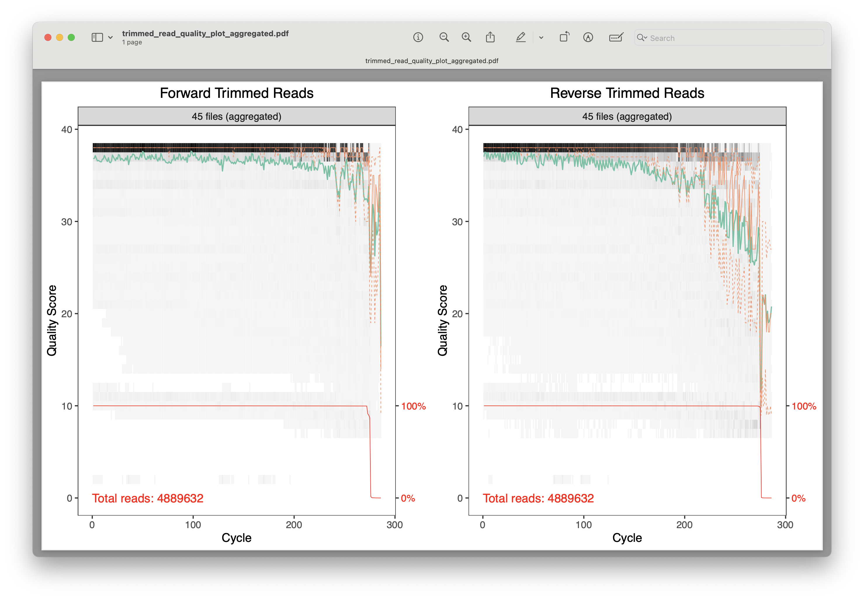
Fig. 18 : A plot of the combined quality scores of all forward and reverse sequence files after primer trimming

4.3.2 Reads retained after primer trimming

Besides the quality scores, we can also calculate the percentage of reads retained after primer trimming. Investigating if a similar proportion of reads are retained across samples, as well as the actual average proportion can help determine issues regarding our code or specific samples.

# Determine percentage retained after primer trimming
metadata$trimming_retained_pct <- round((metadata$trimmed_reads / metadata$raw_reads_f) * 100, 1)
metadata$trimming_retained_pct

Output

> metadata$trimming_retained_pct
 [1] 88.1 88.7 88.1 88.1 88.0 87.8 88.7 89.0 88.3 88.7 88.1 88.2 87.7 62.1 24.0 42.2 36.7 44.0 84.3 87.7 88.1 88.2 88.7 88.1
[25] 88.1 88.2 87.8 88.2 88.1 88.1 87.7 88.5 88.3 88.0 87.9 87.6 88.6 88.6 88.5 89.1 89.4 89.4 88.4 88.1 88.2

Looking at the output, we can see that we observe the same value for sample Akakina_1 as was reported by cutadapt earlier, i.e., 88.1%. As mentioned before, it is always good to double-check if results are as expected! Besides this single value, we can see that most values are in the high 80s, except for a few. Let’s investigate this further.

4.3.3 Visualise read count after primer trimming

Rather than looking at the list of numbers, it can be easier to interpret data by visualising it in a graph. In this case, we can plot a stacked bar chart with the raw read count and trimmed read count. Since the values are stored in our metadata dataframe, we can accomplish this easily using the ggplot2 R package. Let’s create a simple stacked bar chart, as well as a more annotated one to show the power of R and ggplot2.

# Visualise reads after primer trimming
ggplot(metadata, aes(x = sampleID)) +
  geom_bar(aes(y = raw_reads_f, fill = "red"), stat = "identity") +
  geom_bar(aes(y = trimmed_reads, fill = "green"), stat = "identity")
ggsave(filename = file.path("0.metadata", "stacked_bar_raw_trimmed.png"), plot = last_plot(), bg = "white", dpi = 300)

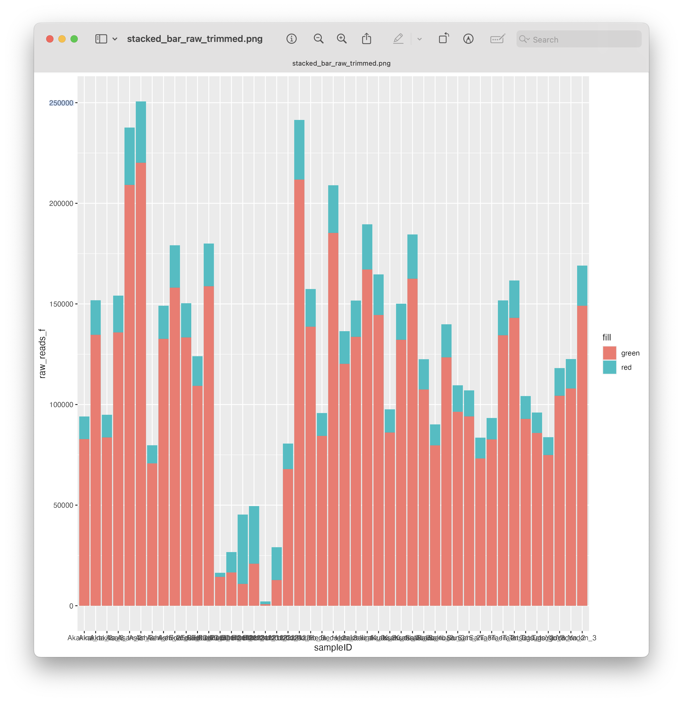
Fig. 19 : A simple stacked bar chart depicting the number of reads before and after primer trimming

As you can see, with only 4 lines of code, we managed to create a simple stacked bar chart and save it to our 0.metadata folder. However, let’s make this look a little bit nicer with some additional formatting and annotations.

# Formatting and annotations to stacked bar chart
ggplot(metadata, aes(x = reorder(sampleID, raw_reads_f))) +
  geom_bar(aes(y = raw_reads_f, fill = "raw_reads"), stat = "identity", width = 0.7) +
  geom_bar(aes(y = trimmed_reads, fill = "trimmed_reads"), stat = "identity", width = 0.7) +
  geom_text(aes(y = raw_reads_f, label = paste0(comma(trimmed_reads), " (", sprintf("%.1f%%", trimming_retained_pct), ")")),
    hjust = -0.1, size = 3, color = "black", position = position_nudge(y = max(metadata$raw_reads_f) * 0.02)) +
  scale_fill_manual(values = c("trimmed_reads" = "#469597", "raw_reads" = "#BBC6C8"), labels = c("Raw read count", "Trimmed read count")) +
  scale_y_continuous(labels = comma, expand = expansion(mult = c(0, 0.2))) +
  coord_flip() +
  labs(title = "Read Counts Before and After Trimming", x = "Sample ID", y = "Number of Reads", fill = "") +
  theme_minimal() +
  theme(legend.position = "top", panel.grid.major.y = element_blank())
ggsave(filename = file.path("0.metadata", "stacked_bar_raw_trimmed_annotated.png"), plot = last_plot(), bg = "white", dpi = 300)

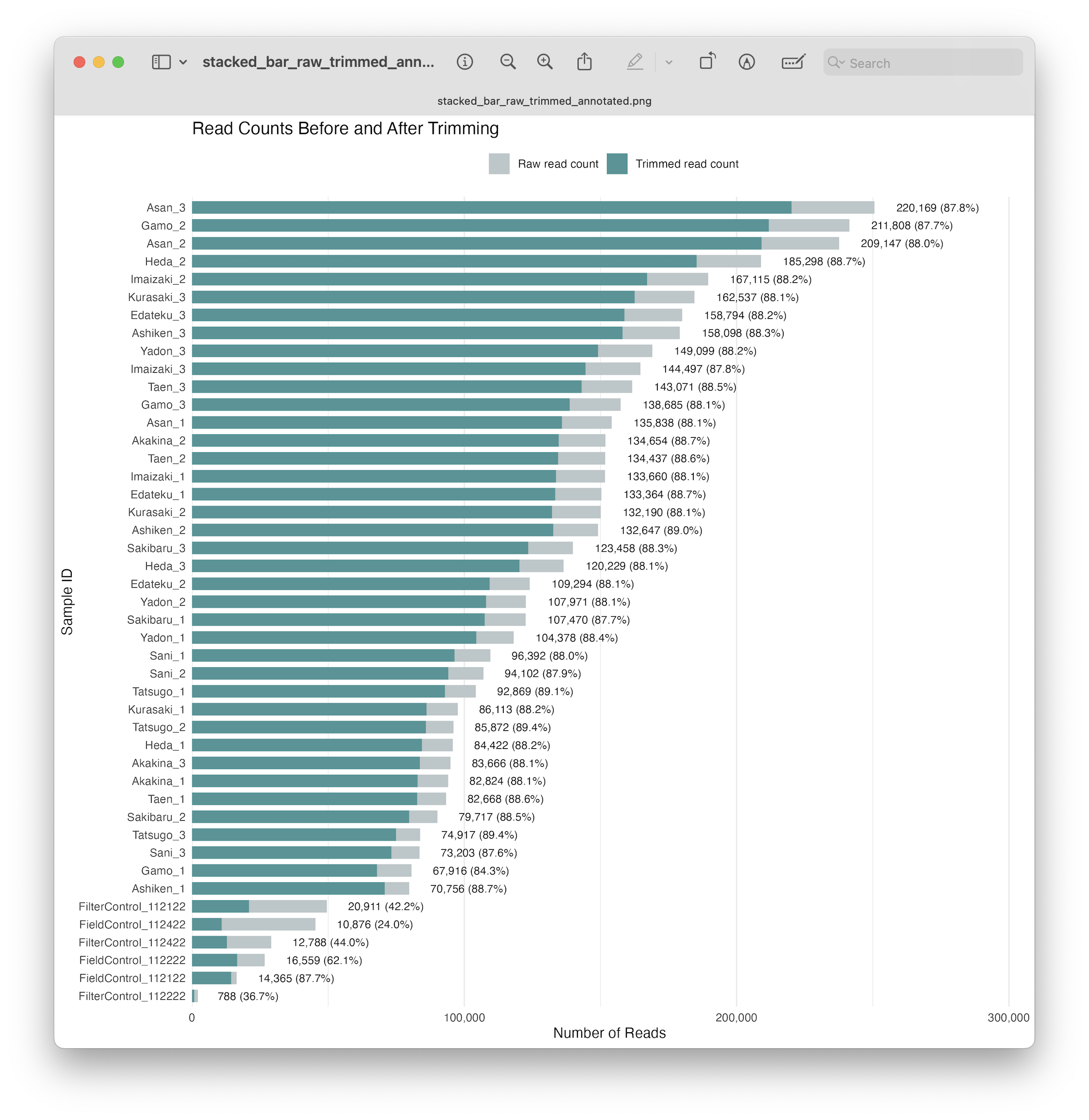
Fig. 20 : A formatted and annotated stacked bar chart depicting the number of reads before and after primer trimming

From this plot, we can see that a similar proportion of reads were retained after primer trimming for all samples, but that some of our negative controls lost a larger proportion of reads. This observation is quite common and fits within the parameters of metabarcoding data, so let’s continue with the analysis.

5. Quality filtering

5.1 Sample processing

During the bioinformatic pipeline, it is critical to only retain high-quality reads to reduce the abundance and impact of spurious sequences. While we conducted some filtering during primer trimming, the quality score plot still indicates additional filtering is needed. There is an intrinsic error rate to all polymerases used during PCR amplification, as well as sequencing technologies. For example, the most frequently used polymerase during PCR is Taq, though lacks 3’ to 5’ exonuclease proofreading activity, resulting in relatively low replication fidelity. These errors will generate some portion of sequences that vary from their biological origin sequence. Such reads can substantially inflate metrics such as alpha diversity, especially in a denoising approach (more on this later). While it is near-impossible to remove all of these sequences bioinformatically, especially PCR errors, we will attempt to remove erroneous reads by filtering on base calling quality scores (the fourth line of a sequence record in a .fastq file).

For quality filtering, we will trim all sequences that do not adhere to a specific set of rules. We will be using the filterAndTrim() function in dada2 for this step. Quality filtering parameters are not standardized, but rather specific for each library. For our tutorial data, we will filter out all sequences that do not adhere to a minimum and maximum length, have unassigned base calls (‘N’), and have a higher expected error than 2. Once we have filtered our data, we can check the quality using the plotQualityProfile() function again and compare it to the previous steps.

Before quality filtering, we need to set some additional variables, including the output folder (in case it does not yet exist) and a list of output files

## Step four: quality filtering
# Set variables
if(!dir.exists("3.filtered")) dir.create("3.filtered")
filtered_forward_reads <- file.path("3.filtered", basename(raw_forward_reads))
filtered_reverse_reads <- file.path("3.filtered", basename(raw_reverse_reads))

Once we have set the variables, we can run the filterAndTrim() function. This function takes a list of input forward reads (trimmed_forward_reads), a list of output forward reads (filtered_forward_reads), a list of input reverse reads (trimmed_reverse_reads), a list of output reverse reads (filtered_reverse_reads), and the filtering parameters, including maxEE for the applied quality filtering threshold, rm.phix to remove any reads that match the PhiX bacteriophage genome (added to metabarcoding libraries to increas complexity), maxN to remove sequences containing unambiguous basecalls, and the truncation and length settings truncLen, truncQ, and minLen.

# perform quality filtering
filtered_out <- filterAndTrim(trimmed_forward_reads, filtered_forward_reads, trimmed_reverse_reads, filtered_reverse_reads,
                              trimLeft = c(0,0), truncLen = c(225,216), maxN = 0, maxEE = c(2,2), truncQ = 2,
                              minLen = 100, rm.phix = TRUE, compress = TRUE, multithread = TRUE)

filtered_out is a named list containing the filenames, as well as a column with initial read counts (reads.in) and a column with read counts after filtering (reads.out). As we did before, let’s add the filtered read count to our metadata file for record keeping.

# add filtering results to metadata file
rownames(filtered_out) <- gsub("_R1_001\\.fastq\\.gz$", "", rownames(filtered_out))
metadata$filtered_reads <- filtered_out[metadata$sampleID, "reads.out"]

5.2 Visualising results

5.2.1 Quality scores

As before, we can visualise the quality scores to determine if filtering was successfull. However, unlike before, let’s generate plots for each sample separately, rather than create one aggregated plot, and sort them by location.

## Step five: check quality filtered files
# Check quality scores across filtering steps
for (location in unique(metadata$sampleLocation)) {
  plot_list <- list()
  location_samples <- metadata %>% filter(sampleLocation == location) %>% pull(sampleID)
  cat("Analysing samples of location", location, "\n")
  for (i in seq_along(location_samples)) {
    f_plot_raw <- plotQualityProfile(file.path("1.raw", paste0(location_samples[i], "_R1_001.fastq.gz")))
    f_plot_trimmed <- plotQualityProfile(file.path("2.trimmed", paste0(location_samples[i], "_R1_001.fastq.gz")))
    f_plot_filtered <- plotQualityProfile(file.path("3.filtered", paste0(location_samples[i], "_R1_001.fastq.gz")))
    r_plot_raw <- plotQualityProfile(file.path("1.raw", paste0(location_samples[i], "_R2_001.fastq.gz")))
    r_plot_trimmed <- plotQualityProfile(file.path("2.trimmed/", paste0(location_samples[i], "_R2_001.fastq.gz")))
    r_plot_filtered <- plotQualityProfile(file.path("3.filtered/", paste0(location_samples[i], "_R2_001.fastq.gz")))
    plot_list[[i]] <- grid.arrange(f_plot_raw, f_plot_trimmed, f_plot_filtered, 
                                   r_plot_raw, r_plot_trimmed, r_plot_filtered, ncol = 6)
  }
  ggsave(filename = file.path("0.metadata", paste0(location, "_quality_profile.png")),
         plot = marrangeGrob(plot_list, nrow = length(plot_list), ncol = 1),
         width = 30, height = 5 * length(plot_list), dpi = 300)
}

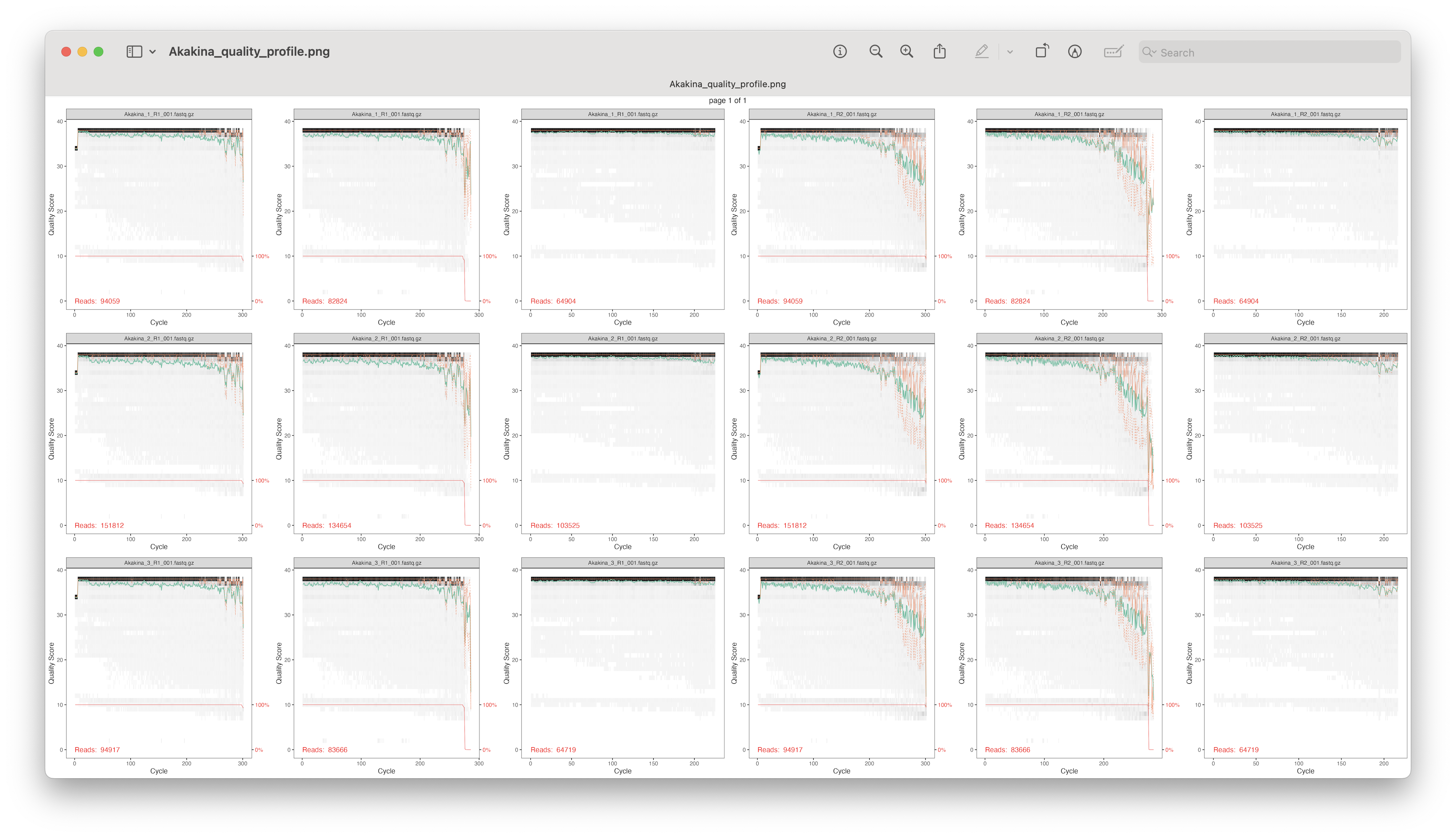
Fig. 21 : Tracked quality scores for location Akakina across all filtering steps for the forward and reverse reads

From this plot, we can track the quality scores for each sample per location across all filtering steps for the forward and reverse reads. As shown in the figure, after the filterAndTrim() function, all quality scores are very high, so we can continue with the analysis and further filtering is not necessary.

5.2.2 Visualise read counts

Similar to what we did to check primer trimming, we can generate a stacked bar plot, now including the number of reads after quality filtering. Note that we first calculate the percentage of reads retained, as before, for printing, as well as the similar code used for plotting.

# Determine percentage retained after quality filtering
metadata$filtering_retained_pct <- round((metadata$filtered_reads / metadata$raw_reads_f) * 100, 1)

# Formatting and annotations to stacked bar chart
ggplot(metadata, aes(x = reorder(sampleID, raw_reads_f))) +
  geom_bar(aes(y = raw_reads_f, fill = "raw_reads"), stat = "identity", width = 0.7) +
  geom_bar(aes(y = trimmed_reads, fill = "trimmed_reads"), stat = "identity", width = 0.7) +
  geom_bar(aes(y = filtered_reads, fill = "filtered_reads"), stat = "identity", width = 0.7) +
  geom_text(aes(y = raw_reads_f, label = paste0(comma(filtered_reads), " (", sprintf("%.1f%%", filtering_retained_pct), ")")),
    hjust = -0.1, size = 3, color = "black", position = position_nudge(y = max(metadata$raw_reads_f) * 0.02)) +
  scale_fill_manual(values = c("trimmed_reads" = "#469597", "raw_reads" = "#BBC6C8", "filtered_reads" = "#DDBEAA"), labels = c("Filtered read count", "Raw read count", "Trimmed read count")) +
  scale_y_continuous(labels = comma, expand = expansion(mult = c(0, 0.2))) +
  coord_flip() +
  labs(title = "Read counts across filtering steps", x = "Sample ID", y = "Number of Reads", fill = "") +
  theme_minimal() +
  theme(legend.position = "top", panel.grid.major.y = element_blank())
ggsave(filename = file.path("0.metadata", "stacked_bar_raw_trimmed_filtered.png"), plot = last_plot(), bg = "white", dpi = 300)

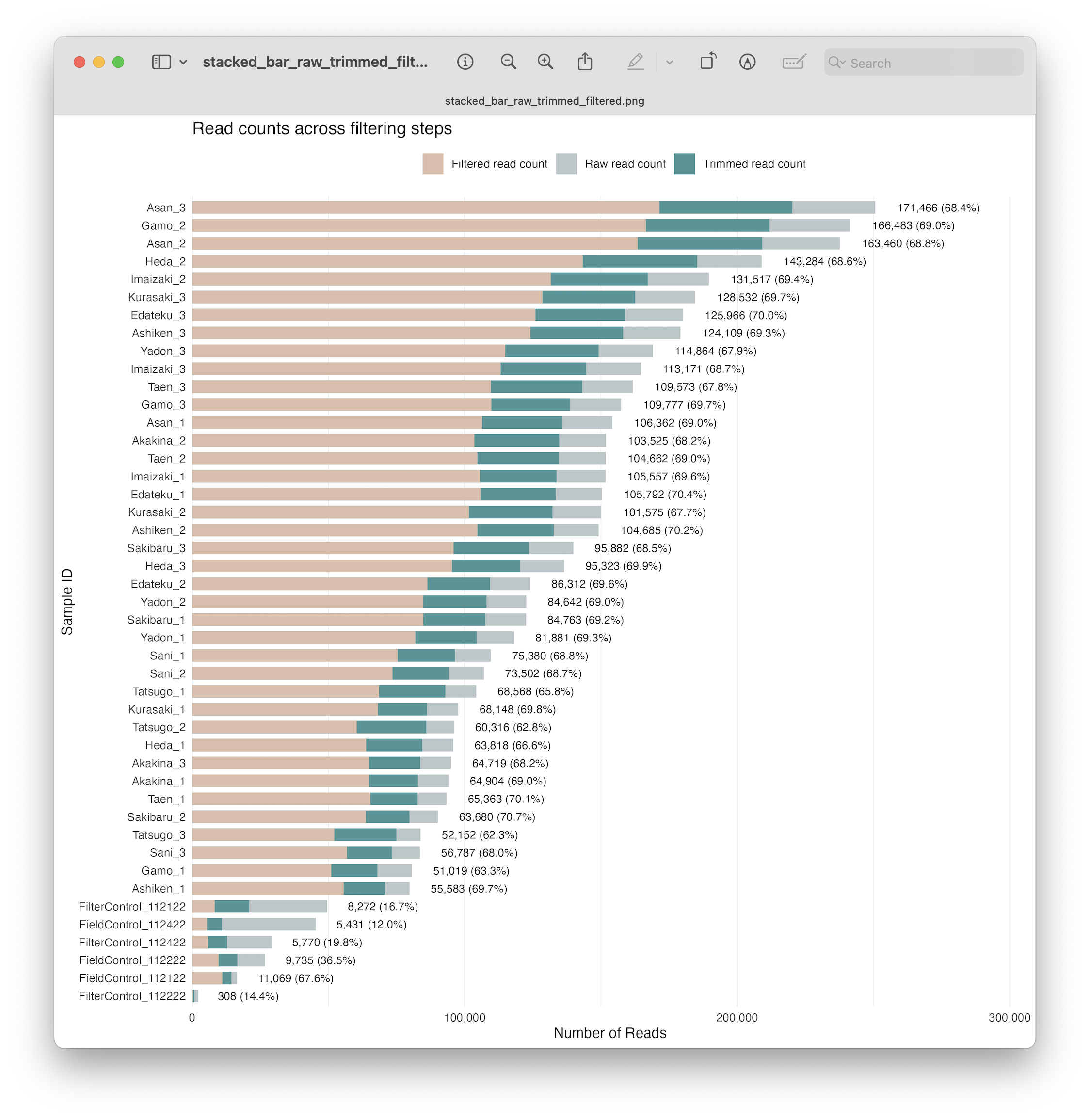
Fig. 22 : A formatted and annotated stacked bar chart depicting the number of reads across filtering steps

6. Learning error rates

Once we have filtered out the low quality data and retained only high quality reads, we can move forward with our bioinformatic pipeline, i.e., generating an error model by learning the specific error-signature of our dataset. Each sequencing run, even when all goes well, will ahve its own subtle variations to its error profile. This step tries to assess that for both the forward and reverse reads, so that we can generate amplicon sequence variants (ASVs) in the next step. We can use the function learnErrors() in dada2 to accomplish this step. I recommend setting the parameter multithread = TRUE, as this is quite a computationally heavy step.

## Step six: learn error rates for our data
# Generate an error model
err_forward_reads <- learnErrors(filtered_forward_reads, multithread = TRUE)
err_reverse_reads <- learnErrors(filtered_reverse_reads, multithread = TRUE)

Output

> err_forward_reads <- learnErrors(filtered_forward_reads, multithread = TRUE)
113168250 total bases in 502970 reads from 5 samples will be used for learning the error rates.
> err_reverse_reads <- learnErrors(filtered_reverse_reads, multithread = TRUE)
108641520 total bases in 502970 reads from 5 samples will be used for learning the error rates.

Dada2 also incorporates a plotting function (plotErrors()) to visualise how well the estimated error rates match with up with the observed. The red line of the graph is the expected error rate based on the quality score, the black line represents the estimate, and the grey dots represent the observed error rates. In general, we want the error frequency (y-axis) to reduce with increased quality scores (y-axis) and that the observed error rates (grey dots) follow the estimated error rates (black line).

# Plot error rates
error_reads_forward_plot <- plotErrors(err_forward_reads, nominalQ = TRUE) + ggplot2::labs(title = "Error Forward")
error_reads_reverse_plot <- plotErrors(err_reverse_reads, nominalQ = TRUE) + ggplot2::labs(title = "Error Reverse")
error_plots <- ggarrange(error_reads_forward_plot, error_reads_reverse_plot, nrow = 2)
ggsave(filename = file.path("0.metadata", "error_plots.pdf"), plot = error_plots, width = 6, height = 10)

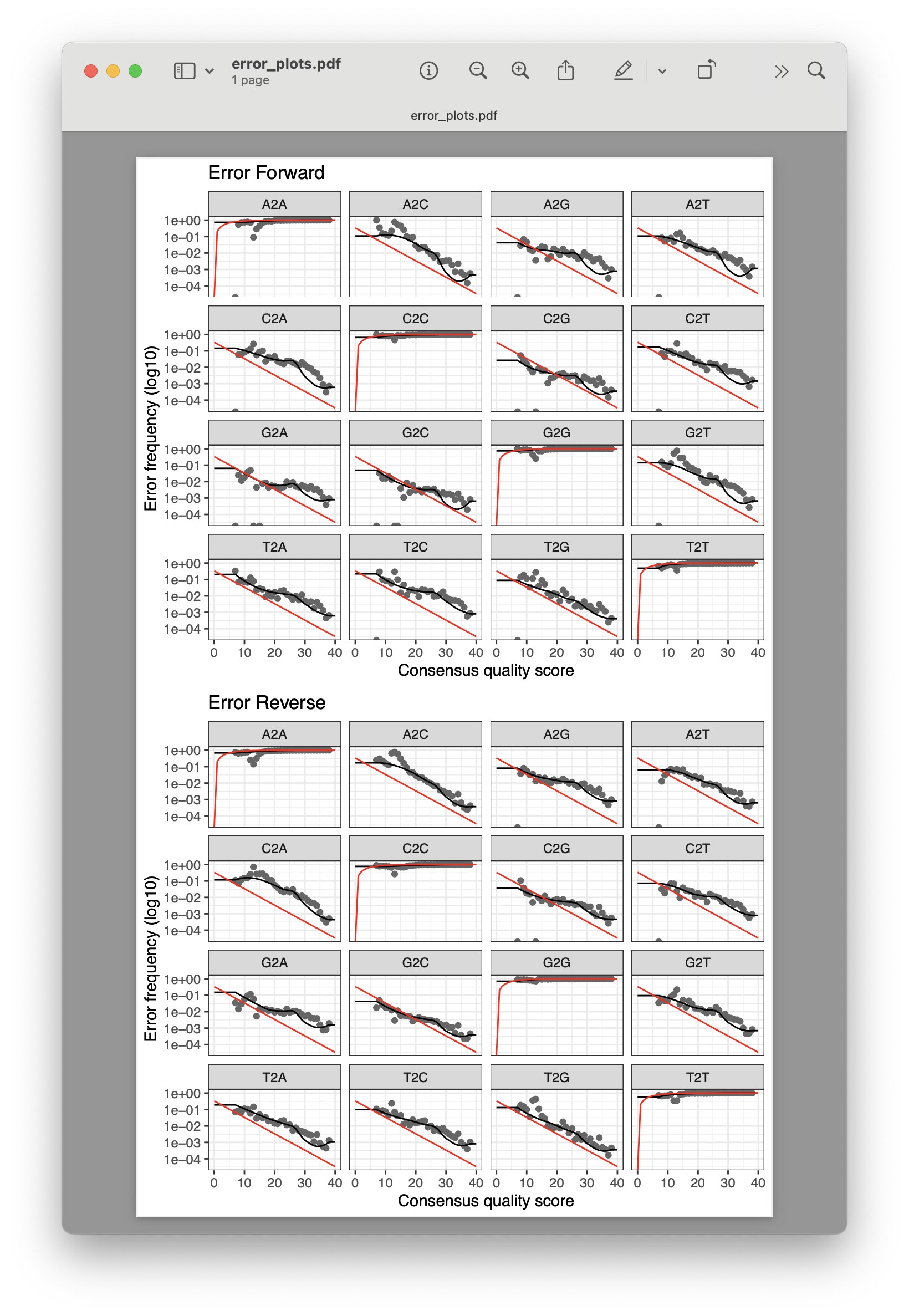
Fig. 23 : The expected (red line), estimated (black line), and observed (grey dots) error rates for our dataset.

7. Generating ASVs

7.1 Denoising the data

Now that our data set is filtered and we’ve learned the error rates, we are ready for the next step in the bioinformatic pipeline, i.e., looking for biologically meaningful or biologically correct sequences. Two approaches exist to achieve this goal, including denoising and clustering. There is still an ongoing debate on what the best approach is to obtain these biologically meaningful sequences. For more information, these are two good papers to read: (Brandt et al., 2021) and (Antich et al., 2021). For this workshop, we won’t be discussing this topic in much detail, but this is the basic idea…

When clustering the dataset, OTUs (Operational Taxonomic Units) will be generated by combining sequences that are similar to a set percentage level (traditionally 97%), with the most abundant sequence identified as the true sequence. When clustering at 97%, this means that if a sequence is more than 3% different than the generated OTU, a second OTU will be generated. The concept of OTU clustering was introduced in the 1960s and has been debated since. Clustering the dataset is usually used for identifying species in metabarcoding data.

Denoising, on the other hand, attempts to identify all correct biological sequences through an algorithm. In short, denoising will cluster the data with a 100% threshold and tries to identify errors based on abundance differences and error profiles. The retained sequences are called ASVs (Amplicon Sequence Variants) or ZOTUs (Zero-radius Operation Taxonomic Unit). Denoising the dataset is usually used for identifying intraspecific variation in metabarcoding data. A schematic of both approaches can be found below.

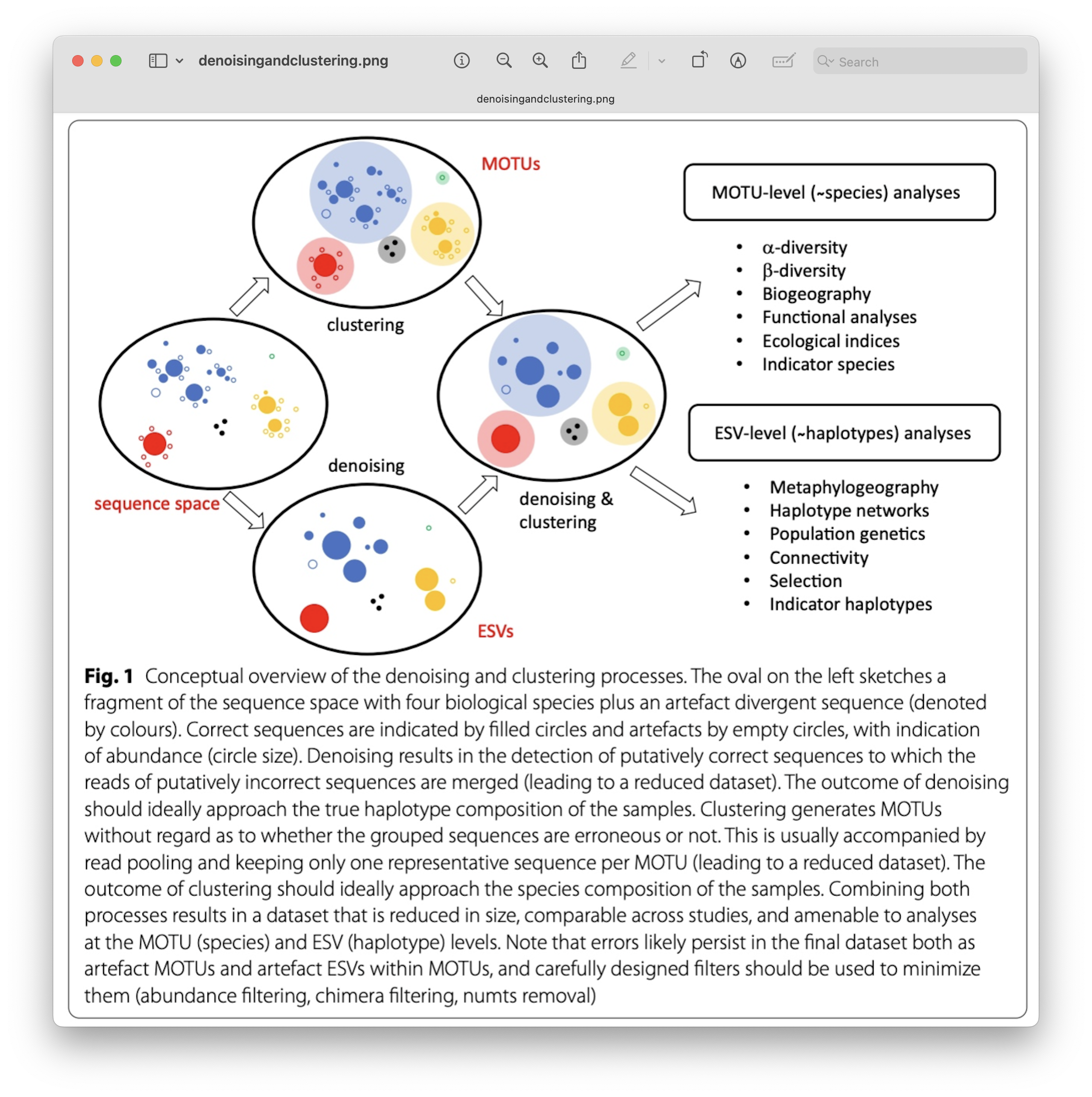
Fig. 24 : A schematic representation of denoising and clustering. Copyright: Antich et al., 2021

This difference in approach may seem small but has a very big impact on your final dataset!

When you denoise the dataset, it is expected that one species may have more than one ASV. This means that when the reference database is incomplete, or you plan to work with ASVs instead of taxonomic assignments, your diversity estimates will be highly inflated. When clustering the dataset, on the other hand, it is expected that an OTU may have more than one species assigned to it, meaning that you may lose some correct biological sequences that are present in your data by merging species with barcodes more similar than 97%. In other words, you will miss out on differentiating closely related species and intraspecific variation.

Since we are following the dada2 pipeline, we will be denoising the data set and infer ASVs based on read abundance and the error profiles we have generated in the previous step. For more information, I recommend reading the dada2 publication.

Dereplication

In the latest versions of dada2, dereplicating the metabarcoding data, i.e., finding unique sequences, does not require a separate step, as it is implemented in the dada() function.

Pooling samples

Interestingly, ASVs can be inferred from each sample separately, but also by combining all samples together using the pool = TRUE parameter. Since this step is computationally intensive, we will not pool the samples for this workshop, but this is something you might want to do for your own data!

## Step seven: generate ASVs
# Infer ASVs using the dada algorithm
dada_forward <- dada(filtered_forward_reads, err = err_forward_reads, pool = FALSE, multithread = TRUE)
dada_reverse <- dada(filtered_reverse_reads, err = err_reverse_reads, pool = FALSE, multithread = TRUE)

Output

> dada_forward <- dada(filtered_forward_reads, err = err_forward_reads, pool = FALSE, multithread = TRUE)
Sample 1 - 64904 reads in 8480 unique sequences.
Sample 2 - 103525 reads in 13912 unique sequences.
Sample 3 - 64719 reads in 7727 unique sequences.
Sample 4 - 106362 reads in 13776 unique sequences.
Sample 5 - 163460 reads in 22246 unique sequences.
Sample 6 - 171466 reads in 18547 unique sequences.
Sample 7 - 55583 reads in 6691 unique sequences.
Sample 8 - 104685 reads in 10538 unique sequences.
Sample 9 - 124109 reads in 13655 unique sequences.
Sample 10 - 105792 reads in 12078 unique sequences.
Sample 11 - 86312 reads in 10089 unique sequences.
Sample 12 - 125966 reads in 14268 unique sequences.
Sample 13 - 11069 reads in 1118 unique sequences.
Sample 14 - 9735 reads in 1180 unique sequences.
Sample 15 - 5431 reads in 865 unique sequences.
Sample 16 - 8272 reads in 1083 unique sequences.
Sample 17 - 308 reads in 73 unique sequences.
Sample 18 - 5770 reads in 761 unique sequences.
Sample 19 - 51019 reads in 5270 unique sequences.
Sample 20 - 166483 reads in 18215 unique sequences.
Sample 21 - 109777 reads in 12073 unique sequences.
Sample 22 - 63818 reads in 6319 unique sequences.
Sample 23 - 143284 reads in 15101 unique sequences.
Sample 24 - 95323 reads in 11985 unique sequences.
Sample 25 - 105557 reads in 11235 unique sequences.
Sample 26 - 131517 reads in 14691 unique sequences.
Sample 27 - 113171 reads in 11752 unique sequences.
Sample 28 - 68148 reads in 8922 unique sequences.
Sample 29 - 101575 reads in 10303 unique sequences.
Sample 30 - 128532 reads in 14843 unique sequences.
Sample 31 - 84763 reads in 9613 unique sequences.
Sample 32 - 63680 reads in 6861 unique sequences.
Sample 33 - 95882 reads in 10886 unique sequences.
Sample 34 - 75380 reads in 9105 unique sequences.
Sample 35 - 73502 reads in 9774 unique sequences.
Sample 36 - 56787 reads in 8489 unique sequences.
Sample 37 - 65363 reads in 7542 unique sequences.
Sample 38 - 104662 reads in 11532 unique sequences.
Sample 39 - 109573 reads in 11254 unique sequences.
Sample 40 - 68568 reads in 10310 unique sequences.
Sample 41 - 60316 reads in 8631 unique sequences.
Sample 42 - 52152 reads in 8201 unique sequences.
Sample 43 - 81881 reads in 10421 unique sequences.
Sample 44 - 84642 reads in 10825 unique sequences.
Sample 45 - 114864 reads in 13894 unique sequences.
> dada_reverse <- dada(filtered_reverse_reads, err = err_reverse_reads, pool = FALSE, multithread = TRUE)
Sample 1 - 64904 reads in 9966 unique sequences.
Sample 2 - 103525 reads in 14506 unique sequences.
Sample 3 - 64719 reads in 9345 unique sequences.
Sample 4 - 106362 reads in 17586 unique sequences.
Sample 5 - 163460 reads in 22977 unique sequences.
Sample 6 - 171466 reads in 24066 unique sequences.
Sample 7 - 55583 reads in 7859 unique sequences.
Sample 8 - 104685 reads in 14191 unique sequences.
Sample 9 - 124109 reads in 18170 unique sequences.
Sample 10 - 105792 reads in 15100 unique sequences.
Sample 11 - 86312 reads in 13004 unique sequences.
Sample 12 - 125966 reads in 16830 unique sequences.
Sample 13 - 11069 reads in 1433 unique sequences.
Sample 14 - 9735 reads in 2359 unique sequences.
Sample 15 - 5431 reads in 1737 unique sequences.
Sample 16 - 8272 reads in 2971 unique sequences.
Sample 17 - 308 reads in 151 unique sequences.
Sample 18 - 5770 reads in 1849 unique sequences.
Sample 19 - 51019 reads in 7735 unique sequences.
Sample 20 - 166483 reads in 20967 unique sequences.
Sample 21 - 109777 reads in 13798 unique sequences.
Sample 22 - 63818 reads in 8731 unique sequences.
Sample 23 - 143284 reads in 19553 unique sequences.
Sample 24 - 95323 reads in 13637 unique sequences.
Sample 25 - 105557 reads in 13256 unique sequences.
Sample 26 - 131517 reads in 18209 unique sequences.
Sample 27 - 113171 reads in 14828 unique sequences.
Sample 28 - 68148 reads in 11521 unique sequences.
Sample 29 - 101575 reads in 11118 unique sequences.
Sample 30 - 128532 reads in 16911 unique sequences.
Sample 31 - 84763 reads in 11360 unique sequences.
Sample 32 - 63680 reads in 8199 unique sequences.
Sample 33 - 95882 reads in 13894 unique sequences.
Sample 34 - 75380 reads in 11080 unique sequences.
Sample 35 - 73502 reads in 10961 unique sequences.
Sample 36 - 56787 reads in 9284 unique sequences.
Sample 37 - 65363 reads in 9197 unique sequences.
Sample 38 - 104662 reads in 15520 unique sequences.
Sample 39 - 109573 reads in 17623 unique sequences.
Sample 40 - 68568 reads in 10510 unique sequences.
Sample 41 - 60316 reads in 9580 unique sequences.
Sample 42 - 52152 reads in 8129 unique sequences.
Sample 43 - 81881 reads in 12792 unique sequences.
Sample 44 - 84642 reads in 13029 unique sequences.
Sample 45 - 114864 reads in 17908 unique sequences.

7.2 Visualising results

Let’s build upon our stacked bar chart and include the read count after denoising. First, we need to extract the read count from the dada objects we created during denoising.

## Step eight: check generated ASVs
# Extract read count from dada objects and add to metadata
dada_f <- sapply(dada_forward, function(x) sum(getUniques(x)))
dada_r <- sapply(dada_reverse, function(x) sum(getUniques(x)))

Next, we need to rename the labels to match the sample IDs rather than file names.

# Rename labels to match sample IDs using regex patterns
names(dada_f) <- gsub("_R1_001\\.fastq\\.gz$", "", names(dada_f))
names(dada_r) <- gsub("_R2_001\\.fastq\\.gz$", "", names(dada_r))

Then, we need to find the minimum value between the read count for the forward and reverse reads.

# Find the minimum value of read count and add to metadata
metadata <- metadata %>%
  mutate(
    denoised_reads = pmin(
      dada_f[match(sampleID, names(dada_f))],
      dada_r[match(sampleID, names(dada_r))]))

Once we have the read counts, we can calculate the percentage as before and plot the data.

# Determine percentage retained after denoising
metadata$denoising_retained_pct <- round((metadata$denoised_reads / metadata$raw_reads_f) * 100, 1)

# Formatting and annotations to stacked bar chart
ggplot(metadata, aes(x = reorder(sampleID, raw_reads_f))) +
  geom_bar(aes(y = raw_reads_f, fill = "raw_reads"), stat = "identity", width = 0.7) +
  geom_bar(aes(y = trimmed_reads, fill = "trimmed_reads"), stat = "identity", width = 0.7) +
  geom_bar(aes(y = filtered_reads, fill = "filtered_reads"), stat = "identity", width = 0.7) +
  geom_bar(aes(y = denoised_reads, fill = "denoised_reads"), stat = "identity", width = 0.7) +
  geom_text(aes(y = raw_reads_f, label = paste0(comma(denoised_reads), " (", sprintf("%.1f%%", denoising_retained_pct), ")")),
    hjust = -0.1, size = 3, color = "black", position = position_nudge(y = max(metadata$raw_reads_f) * 0.02)) +
  scale_fill_manual(values = c("trimmed_reads" = "#469597", "raw_reads" = "#BBC6C8", "filtered_reads" = "#DDBEAA", "denoised_reads" = "#806491"), labels = c("Denoised read count", "Filtered read count", "Raw read count", "Trimmed read count")) +
  scale_y_continuous(labels = comma, expand = expansion(mult = c(0, 0.2))) +
  coord_flip() +
  labs(title = "Read counts across filtering steps", x = "Sample ID", y = "Number of Reads", fill = "") +
  theme_minimal() +
  theme(legend.position = "top", panel.grid.major.y = element_blank())
ggsave(filename = file.path("0.metadata", "stacked_bar_raw_trimmed_filtered_denoised.png"), plot = last_plot(), bg = "white", dpi = 300)

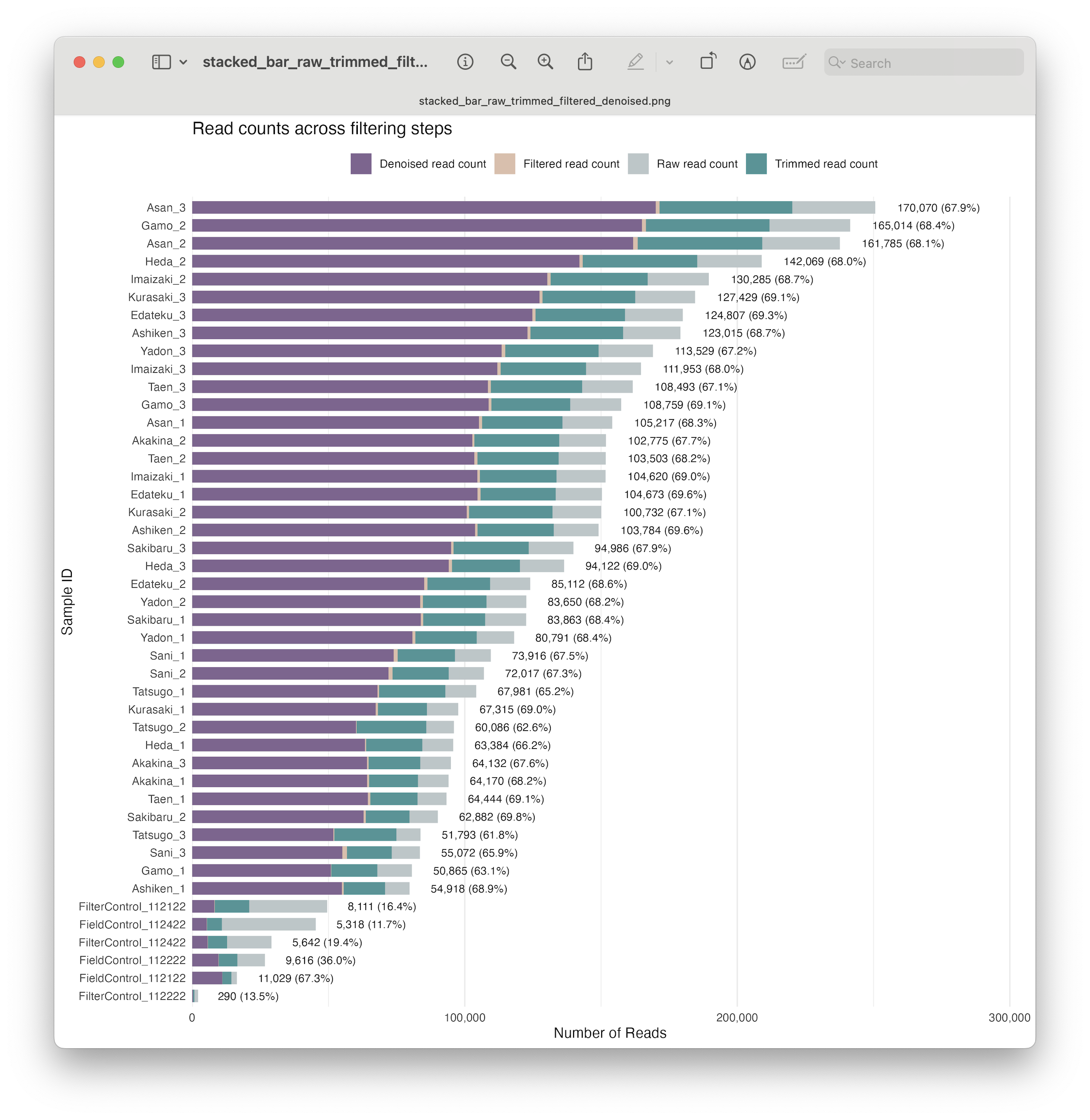
Fig. 25 : A formatted and annotated stacked bar chart depicting the number of reads across filtering steps, including denoising

8. Merging forward and reverse reads

8.1 Reconstruct the full amplicon

Now that we have our ASVs, we can merge the forward and reverse reads in our data to reconstruct the full amplicon. We can merge reads using the mergePairs() function in the dada2 R package. Merging forward and reverse reads works by the Needleman-Wunsch algorithm. By default, a successful alignment requirs an overlap of at least 12 basepairs (minOverlap), as well as 0 mismatches (maxMismatch). However, for our data, we will set these parameters to 10 and 2, respectively. Also, we can set the trimOverhang = TRUE parameter in case any of the reads go passed their opposite primers (this should not be the case, however, given the amplicon length and the primer trimming we performed with cutadapt).

## Step nine: merge forward and reverse reads
merged_amplicons <- mergePairs(dada_forward, filtered_forward_reads, dada_reverse, filtered_reverse_reads,
                               minOverlap = 10, maxMismatch = 2, trimOverhang = TRUE, verbose = TRUE)

Output

> merged_amplicons <- mergePairs(dada_forward, filtered_forward_reads, dada_reverse, filtered_reverse_reads,
+                                minOverlap = 10, maxMismatch = 2, trimOverhang = TRUE, verbose = TRUE)
63905 paired-reads (in 481 unique pairings) successfully merged out of 64011 (in 526 pairings) input.
Duplicate sequences in merged output.
102341 paired-reads (in 532 unique pairings) successfully merged out of 102506 (in 590 pairings) input.
Duplicate sequences in merged output.
63809 paired-reads (in 419 unique pairings) successfully merged out of 63910 (in 466 pairings) input.
Duplicate sequences in merged output.
104535 paired-reads (in 895 unique pairings) successfully merged out of 104806 (in 998 pairings) input.
Duplicate sequences in merged output.
160432 paired-reads (in 1120 unique pairings) successfully merged out of 161048 (in 1318 pairings) input.
Duplicate sequences in merged output.
169231 paired-reads (in 1110 unique pairings) successfully merged out of 169546 (in 1250 pairings) input.
Duplicate sequences in merged output.
54543 paired-reads (in 457 unique pairings) successfully merged out of 54699 (in 516 pairings) input.
Duplicate sequences in merged output.
103161 paired-reads (in 647 unique pairings) successfully merged out of 103453 (in 744 pairings) input.
Duplicate sequences in merged output.
122118 paired-reads (in 855 unique pairings) successfully merged out of 122531 (in 981 pairings) input.
Duplicate sequences in merged output.
103894 paired-reads (in 904 unique pairings) successfully merged out of 104250 (in 1034 pairings) input.
Duplicate sequences in merged output.
84278 paired-reads (in 734 unique pairings) successfully merged out of 84613 (in 835 pairings) input.
Duplicate sequences in merged output.
124047 paired-reads (in 1016 unique pairings) successfully merged out of 124343 (in 1130 pairings) input.
Duplicate sequences in merged output.
11026 paired-reads (in 33 unique pairings) successfully merged out of 11026 (in 33 pairings) input.
Duplicate sequences in merged output.
9609 paired-reads (in 40 unique pairings) successfully merged out of 9609 (in 40 pairings) input.
Duplicate sequences in merged output.
5235 paired-reads (in 22 unique pairings) successfully merged out of 5315 (in 24 pairings) input.
Duplicate sequences in merged output.
7975 paired-reads (in 26 unique pairings) successfully merged out of 8103 (in 29 pairings) input.
286 paired-reads (in 6 unique pairings) successfully merged out of 286 (in 6 pairings) input.
5606 paired-reads (in 27 unique pairings) successfully merged out of 5637 (in 30 pairings) input.
Duplicate sequences in merged output.
50696 paired-reads (in 161 unique pairings) successfully merged out of 50830 (in 169 pairings) input.
Duplicate sequences in merged output.
164020 paired-reads (in 1139 unique pairings) successfully merged out of 164469 (in 1303 pairings) input.
Duplicate sequences in merged output.
108217 paired-reads (in 890 unique pairings) successfully merged out of 108476 (in 987 pairings) input.
Duplicate sequences in merged output.
63111 paired-reads (in 351 unique pairings) successfully merged out of 63260 (in 397 pairings) input.
141414 paired-reads (in 866 unique pairings) successfully merged out of 141724 (in 948 pairings) input.
Duplicate sequences in merged output.
93352 paired-reads (in 1092 unique pairings) successfully merged out of 93662 (in 1211 pairings) input.
Duplicate sequences in merged output.
104131 paired-reads (in 699 unique pairings) successfully merged out of 104303 (in 771 pairings) input.
Duplicate sequences in merged output.
129513 paired-reads (in 783 unique pairings) successfully merged out of 129905 (in 909 pairings) input.
Duplicate sequences in merged output.
111377 paired-reads (in 645 unique pairings) successfully merged out of 111691 (in 718 pairings) input.
Duplicate sequences in merged output.
66827 paired-reads (in 606 unique pairings) successfully merged out of 67019 (in 664 pairings) input.
Duplicate sequences in merged output.
100425 paired-reads (in 520 unique pairings) successfully merged out of 100541 (in 574 pairings) input.
Duplicate sequences in merged output.
126806 paired-reads (in 856 unique pairings) successfully merged out of 127068 (in 962 pairings) input.
Duplicate sequences in merged output.
83417 paired-reads (in 555 unique pairings) successfully merged out of 83526 (in 602 pairings) input.
Duplicate sequences in merged output.
62608 paired-reads (in 423 unique pairings) successfully merged out of 62683 (in 454 pairings) input.
Duplicate sequences in merged output.
94431 paired-reads (in 575 unique pairings) successfully merged out of 94715 (in 640 pairings) input.
Duplicate sequences in merged output.
73538 paired-reads (in 1054 unique pairings) successfully merged out of 73613 (in 1090 pairings) input.
Duplicate sequences in merged output.
71536 paired-reads (in 1024 unique pairings) successfully merged out of 71663 (in 1071 pairings) input.
Duplicate sequences in merged output.
54618 paired-reads (in 959 unique pairings) successfully merged out of 54741 (in 995 pairings) input.
Duplicate sequences in merged output.
64036 paired-reads (in 548 unique pairings) successfully merged out of 64197 (in 597 pairings) input.
Duplicate sequences in merged output.
103004 paired-reads (in 830 unique pairings) successfully merged out of 103221 (in 904 pairings) input.
Duplicate sequences in merged output.
107782 paired-reads (in 802 unique pairings) successfully merged out of 108086 (in 896 pairings) input.
Duplicate sequences in merged output.
67776 paired-reads (in 312 unique pairings) successfully merged out of 67848 (in 342 pairings) input.
Duplicate sequences in merged output.
59906 paired-reads (in 252 unique pairings) successfully merged out of 60013 (in 290 pairings) input.
Duplicate sequences in merged output.
51656 paired-reads (in 257 unique pairings) successfully merged out of 51728 (in 284 pairings) input.
Duplicate sequences in merged output.
80233 paired-reads (in 747 unique pairings) successfully merged out of 80438 (in 811 pairings) input.
Duplicate sequences in merged output.
83003 paired-reads (in 790 unique pairings) successfully merged out of 83284 (in 876 pairings) input.
Duplicate sequences in merged output.
112873 paired-reads (in 1052 unique pairings) successfully merged out of 113147 (in 1167 pairings) input.
Duplicate sequences in merged output.

8.2 Visualising results

Similarly to the previous steps, we can build upon the stacked bar chart to add the read counts after merging.

## Step ten: check merging success
# Extract read count from merged_amplicons and add to metadata
merged_count <- sapply(merged_amplicons, function(x) sum(getUniques(x)))
names(merged_count) <- gsub("_R1_001\\.fastq\\.gz$", "", names(merged_count))
metadata <- metadata %>%
  mutate(merged_reads = merged_count[match(sampleID, names(merged_count))])

# Determine percentage retained after merging
metadata$merging_retained_pct <- round((metadata$merged_reads / metadata$raw_reads_f) * 100, 1)

# Formatting and annotations to stacked bar chart
ggplot(metadata, aes(x = reorder(sampleID, raw_reads_f))) +
  geom_bar(aes(y = raw_reads_f, fill = "raw_reads"), stat = "identity", width = 0.7) +
  geom_bar(aes(y = trimmed_reads, fill = "trimmed_reads"), stat = "identity", width = 0.7) +
  geom_bar(aes(y = filtered_reads, fill = "filtered_reads"), stat = "identity", width = 0.7) +
  geom_bar(aes(y = denoised_reads, fill = "denoised_reads"), stat = "identity", width = 0.7) +
  geom_bar(aes(y = denoised_reads, fill = "merged_reads"), stat = "identity", width = 0.7) +
  geom_text(aes(y = raw_reads_f, label = paste0(comma(merged_reads), " (", sprintf("%.1f%%", merging_retained_pct), ")")),
    hjust = -0.1, size = 3, color = "black", position = position_nudge(y = max(metadata$raw_reads_f) * 0.02)) +
  scale_fill_manual(values = c("trimmed_reads" = "#469597", "raw_reads" = "#BBC6C8", "filtered_reads" = "#DDBEAA", "denoised_reads" = "#806491", "merged_reads" = "#2F70AF"), 
  labels = c("Denoised read count", "Filtered read count", "Merged read count", "Raw read count", "Trimmed read count")) +
  scale_y_continuous(labels = comma, expand = expansion(mult = c(0, 0.2))) +
  coord_flip() +
  labs(title = "Read counts across filtering steps", x = "Sample ID", y = "Number of Reads", fill = "") +
  theme_minimal() +
  theme(legend.position = "top", panel.grid.major.y = element_blank())
ggsave(filename = file.path("0.metadata", "stacked_bar_raw_trimmed_filtered_denoised_merged.png"), plot = last_plot(), bg = "white", dpi = 300)

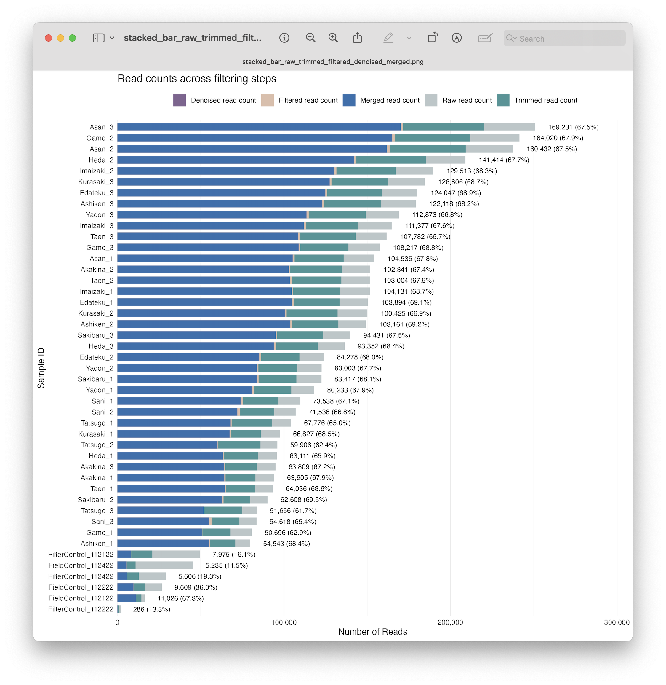
Fig. 26 : A formatted and annotated stacked bar chart depicting the number of reads across filtering steps, including denoising and merging

9. Count table

Once reads are merged, we can generate a count table with the makeSequenceTable() function in the dada2 R package. Using the dim() function, we can investigate the dimensions of the table, which represents the number of samples (45) and number of ASVs (9,313).

## Step 11: construct a count table
count_table <- makeSequenceTable(merged_amplicons)
dim(count_table)

Output

> dim(count_table)
[1]   45 9313

10. Chimera removal

As a final step in our bioinformatic pipeline, we need to remove chimeric sequences. Amplicon sequencing has the potential to generate chimeric reads, which can cause spurious inference of biological variation. Chimeric amplicons form when an incomplete DNA strand anneals to a different template and primes synthesis of a new template derived from two different biological sequences, or in other words chimeras are artefact sequences formed by two or more biological sequences incorrectly joined together. More information can be found in this paper and a simple illustration can be found below.

Fig. 27 : A schematic representation of chimera formation. Copyright: Genome Research

Dada2 identifies likely chimeras by aligning each sequence with those that were recovered in greater abundance and then determining if any lower-abundance sequences can be made exactly by mixing left and right portions of two of the more abundant ones. Dada2 accomplishes this by the column names, which are currently our ASV sequences, and column sums to gather information on abundance.

## Step 12: removing chimeras
count_table_nochimeras <- removeBimeraDenovo(count_table, method = "consensus", multithread = TRUE, verbose = TRUE)

Output

> count_table_nochimeras <- removeBimeraDenovo(count_table, method = "consensus", multithread = TRUE, verbose = TRUE)
Identified 999 bimeras out of 9313 input sequences.

11. Read count tracking

Now that we have finalised our bioinformatic pipeline, we can finish the stacked bar chart by incorporating the read counts after chimera removal.

## Step 13: check chimera removal numbers
# Extract read count per sample and add to metadata
non_chimera_count <- rowSums(count_table_nochimeras)
names(non_chimera_count) <- gsub("_R1_001\\.fastq\\.gz$", "", names(non_chimera_count))
metadata <- metadata %>%
  mutate(nonchimera_reads = non_chimera_count[match(sampleID, names(non_chimera_count))])

# Determine percentage retained after merging
metadata$nonchimera_retained_pct <- round((metadata$nonchimera_reads / metadata$raw_reads_f) * 100, 1)

# Formatting and annotations to stacked bar chart
ggplot(metadata, aes(x = reorder(sampleID, raw_reads_f))) +
  geom_bar(aes(y = raw_reads_f, fill = "raw_reads"), stat = "identity", width = 0.7) +
  geom_bar(aes(y = trimmed_reads, fill = "trimmed_reads"), stat = "identity", width = 0.7) +
  geom_bar(aes(y = filtered_reads, fill = "filtered_reads"), stat = "identity", width = 0.7) +
  geom_bar(aes(y = denoised_reads, fill = "denoised_reads"), stat = "identity", width = 0.7) +
  geom_bar(aes(y = denoised_reads, fill = "merged_reads"), stat = "identity", width = 0.7) +
  geom_bar(aes(y = nonchimera_reads, fill = "nonchimera_reads"), stat = "identity", width = 0.7) +
  geom_text(aes(y = raw_reads_f, label = paste0(comma(nonchimera_reads), " (", sprintf("%.1f%%", nonchimera_retained_pct), ")")),
    hjust = -0.1, size = 3, color = "black", position = position_nudge(y = max(metadata$raw_reads_f) * 0.02)) +
  scale_fill_manual(values = c("trimmed_reads" = "#469597", "raw_reads" = "#BBC6C8", "filtered_reads" = "#DDBEAA", "denoised_reads" = "#806491", "merged_reads" = "#2F70AF", "nonchimera_reads" = "#5F021F"), 
  labels = c("Denoised read count", "Filtered read count", "Merged read count", "Non chimera read count", "Raw read count", "Trimmed read count")) +
  scale_y_continuous(labels = comma, expand = expansion(mult = c(0, 0.2))) +
  coord_flip() +
  labs(title = "Read counts across filtering steps", x = "Sample ID", y = "Number of Reads", fill = "") +
  theme_minimal() +
  theme(legend.position = "top", panel.grid.major.y = element_blank())
ggsave(filename = file.path("0.metadata", "stacked_bar_raw_trimmed_filtered_denoised_merged_nonchimera.png"), plot = last_plot(), bg = "white", dpi = 300)

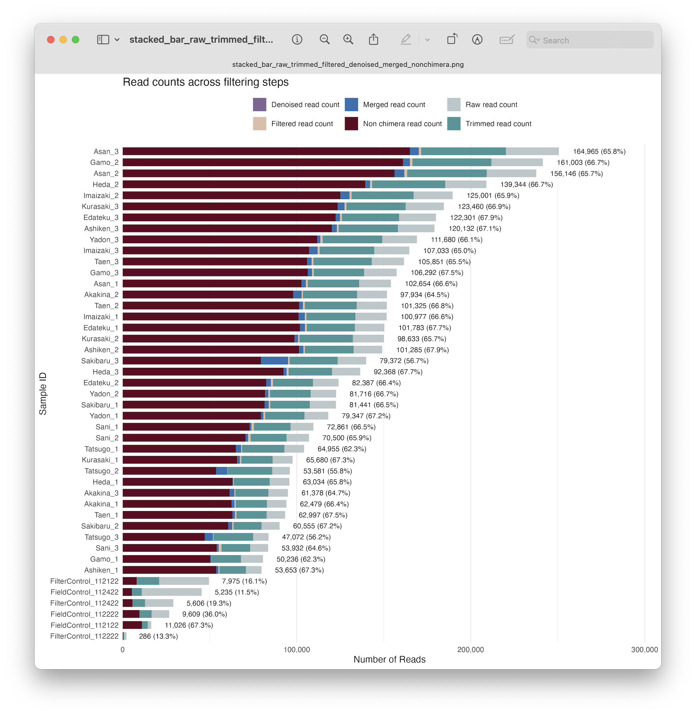
Fig. 28 : A formatted and annotated stacked bar chart depicting the number of reads across filtering steps, including denoising, merging, and chimera removal

12. Saving output files

Before we end the day, it is best to reformat our output and save the files.

## Step 13: Saving output files
# Create directory
if(!dir.exists("4.results")) dir.create("4.results")
# Export metadata file
write.table(metadata, file.path("4.results", "metadata.txt"), quote = FALSE, sep = "\t", row.names = FALSE)
# Change ASV IDs
asv_ids <- paste0("ASV_", seq_along(colnames(count_table_nochimeras)))
names(asv_ids) <- colnames(count_table_nochimeras)
# Export ASV sequences
uniquesToFasta(getUniques(count_table_nochimeras), fout = file.path("4.results","asvs.fasta"),
               ids = asv_ids[colnames(count_table_nochimeras)])
# Export count table
colnames(count_table_nochimeras) <- asv_ids[colnames(count_table_nochimeras)]
rownames(count_table_nochimeras) <- gsub("_R1_001\\.fastq\\.gz$", "", rownames(count_table_nochimeras))
count_table_nochimeras <- as.data.frame(t(count_table_nochimeras))
count_table_nochimeras <- cbind(sampleID = rownames(count_table_nochimeras), count_table_nochimeras)
write.table(t(count_table_nochimeras), file.path("4.results", "count_table.txt"), quote = FALSE, sep = "\t", row.names = FALSE)

Today, we have generated three files, including:

1. an updated metadata file containing read count information across the different steps of the bioinformatic pipeline

2. an ASV fasta file containing a list of all ASVs

3. a count table containing information on read abundance for each ASV per sample

That’s it for today, we will see you tomorrow when we will be creating custom reference databases and assigning a taxonomic ID to our ASVs!