Phylogenetic tree

1. Introduction

Before conducting the statistical analysis, there is one last output file we can create to help us explore our data: a phylogenetic tree of the ASV sequences. Phylogenetic relatedness is commonly used to inform downstream analyses, especially the calculation of phylogeny-aware distnances.

There are many different ways of building phylogenetic trees, ranging from fast heuristic distance-based methods with potential low accuracy (neighbour-joining; NJ) to slow probabilistic model-based highly-accurate methods (Bayesian Inference) and options in between (maximum likelyhood [ML] and maximum parsimony [MP]). The discussion and amount of research conducted on best approaches is vast and, unfortunately, outside the scope of this tutorial. Today, we will show you how to build Bayesian phylogenetic trees using BEAST 2 (Bayesian Evolutionary Analysis by Sampling Trees).

BEAST 2 is a cross-platform program for Bayesian phylogenetic analysis of molecular sequences. It estiamtes rooted, time-measured phylogenies using strict or relaxed molecular clock models. It can be used as a method of reocnstructing phylogenies, but is also a framework for testing evolutionary hypotheses without conditioning on a single tree topology. BEAST 2 uses Markov chain Monte Carlo (MCMC) to average over tree space, so that each tree is weighted proportional to its posterior probability. BEAST 2 includes a graphical user-interface for setting up standard analyses and a suit of programs for analysing the results.

R and GUI

While BEAST 2 comes with a graphical user interface (GUI), we will still have to conduct the first couple of steps of the analysis in R.

2. Multiple Sequence Alignment

To start the analysis, we have to align all our ASV sequences through a multiple sequence alignment (MSA). There are multiple programs capable of creating multiple sequence alignments. Since our pipeline is mainly based in the R environment, we’ll use the AlignSeqs() function of the DECIPHER R package.

First, let’s start RStudio, open a new R script, save it as phylogenetic_tree.R in the bootcamp directory, prepare the R environment.

## set up the working environment
setwd(file.path(Sys.getenv("HOME"), "Desktop", "bootcamp"))
list.files()

## load necessary R packages
for (pkg in c("Biostrings", "DECIPHER", "ape")) {
  if (!require(pkg, character.only = TRUE)) install.packages(pkg)
  library(pkg, character.only = TRUE)
  cat(pkg, "version:", as.character(packageVersion(pkg)), "\n")
}

Once we have loaded all the necessary R packages and set the current working directory, we can read the ASV sequence file (asvs_filtered.fasta) into R.

## read data into R using Biostrings
sequences <- readDNAStringSet(file.path("4.results", "asvs_filtered.fasta"))

Next, we can generate the MSA using the AlignSeqs() function.

## generate alignment using DECIPHER
alignment <- AlignSeqs(sequences, anchor = NA, iterations = 5, refinements = 5)

Output

Determining distance matrix based on shared 8-mers:
  |===================================================================================================================| 100%

Time difference of 15.77 secs

Clustering into groups by similarity:
  |===================================================================================================================| 100%

Time difference of 0.33 secs

Aligning Sequences:
  |===================================================================================================================| 100%

Time difference of 6.92 secs

Iteration 1 of 5:

Determining distance matrix based on alignment:
  |===================================================================================================================| 100%

Time difference of 1.02 secs

Reclustering into groups by similarity:
  |===================================================================================================================| 100%

Time difference of 0.25 secs

Realigning Sequences:
  |===================================================================================================================| 100%

Time difference of 2.51 secs

Iteration 2 of 5:

Determining distance matrix based on alignment:
  |===================================================================================================================| 100%

Time difference of 1.04 secs

Reclustering into groups by similarity:
  |===================================================================================================================| 100%

Time difference of 0.17 secs

Realigning Sequences:
  |===================================================================================================================| 100%

Time difference of 0.37 secs

Iteration 3 of 5:

Determining distance matrix based on alignment:
  |===================================================================================================================| 100%

Time difference of 1.06 secs

Reclustering into groups by similarity:
  |===================================================================================================================| 100%

Time difference of 0.18 secs

Realigning Sequences:
  |===================================================================================================================| 100%

Time difference of 0.2 secs

Alignment converged - skipping remaining iterations.

Refining the alignment:
  |===================================================================================================================| 100%

Time difference of 0.2 secs

Alignment converged - skipping remaining refinements.

Once we have created the MSA, we need to export the alignment. It is important to export the alignment in nexus format, as this is required for the next step. We can use the write.nexus.data() function of the ape R package.

## export alignment in nexus format using ape
write.nexus.data(alignment, file.path("6.phylotree", "asvs_aligned.nex"))

3. BEAUti 2

After we exported the MSA into nexus format, we need to generate an xml document that can be imported into BEAST 2. Luckily, the BEAST 2 developers have created BEAUti 2 (Bayesian Evolutionary Analysis Utility), a GUI that can import a nexus document (the one we just created in the previous step: asvs_aligned.nex) and export the necessary xml document for BEAST 2. After opening the BEAUti 2 app, we need to click the File --> Import Alignment button. Next, we need to navigate to our nexus alignment and click on Open.

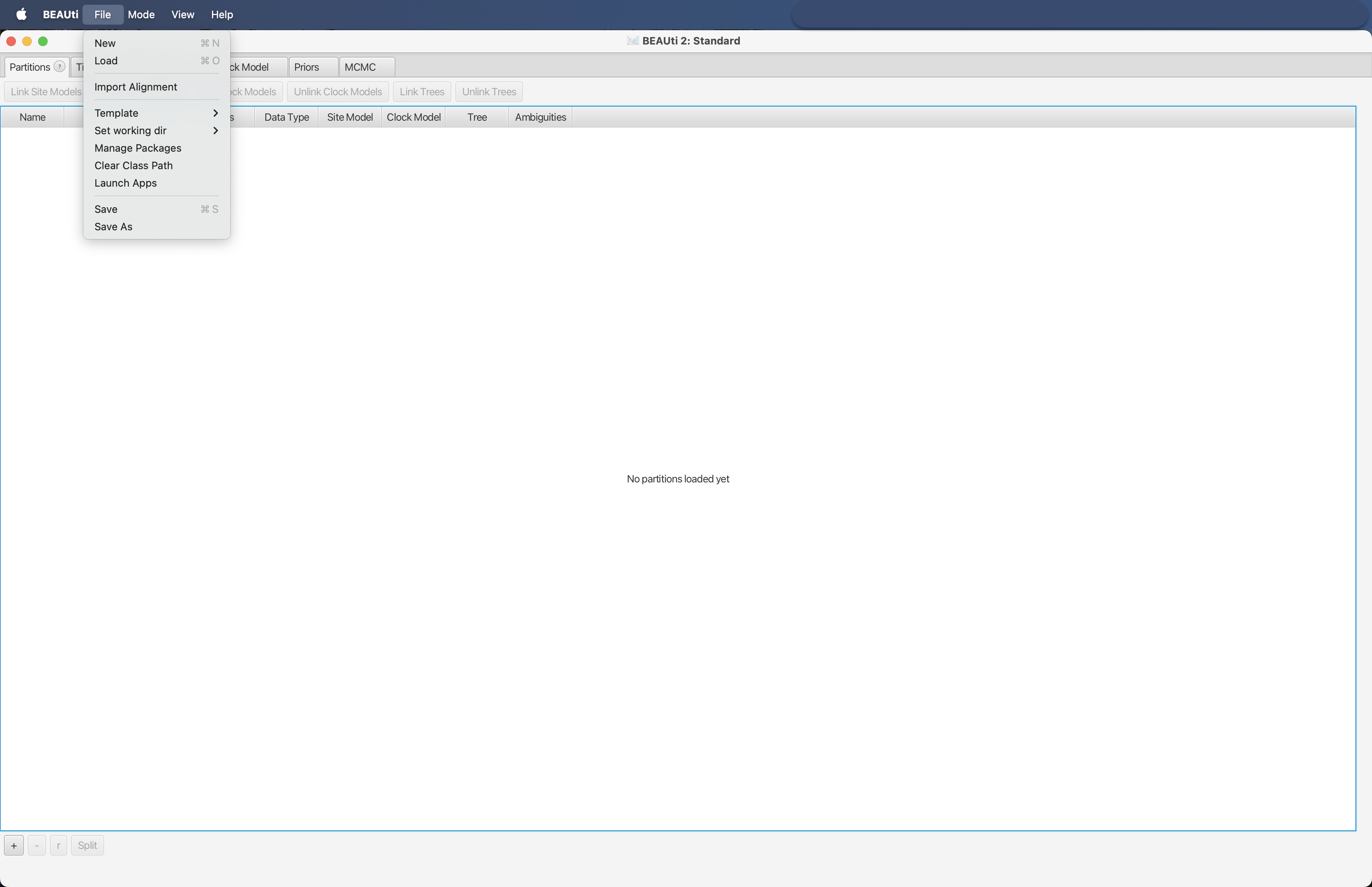
Fig. 51 : Screenshot showing the process of importing a nexus alignment into BEAUti 2.

Once the nexus document is imported, we can change the name under Clock Model and Tree in the Partitions panel (starting window after import). We will set the names from the file name to clock and tree respectively to keep things simple.

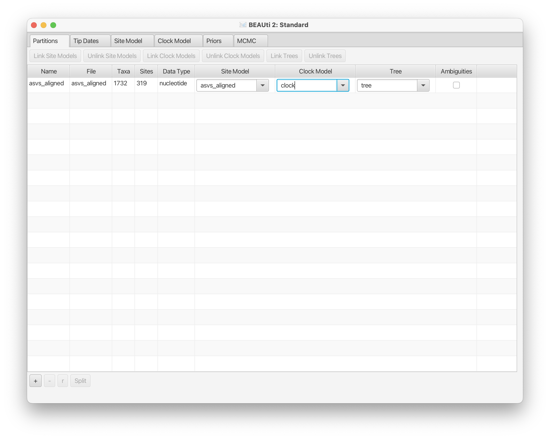
Fig. 52 : Screenshot showing how to change names in BEAUti 2.

Next, we will change the substitution model (Subst Model) in the Site Model panel from JC69 to HKY and leave the Kappa and Frequencies variables to the default settings.

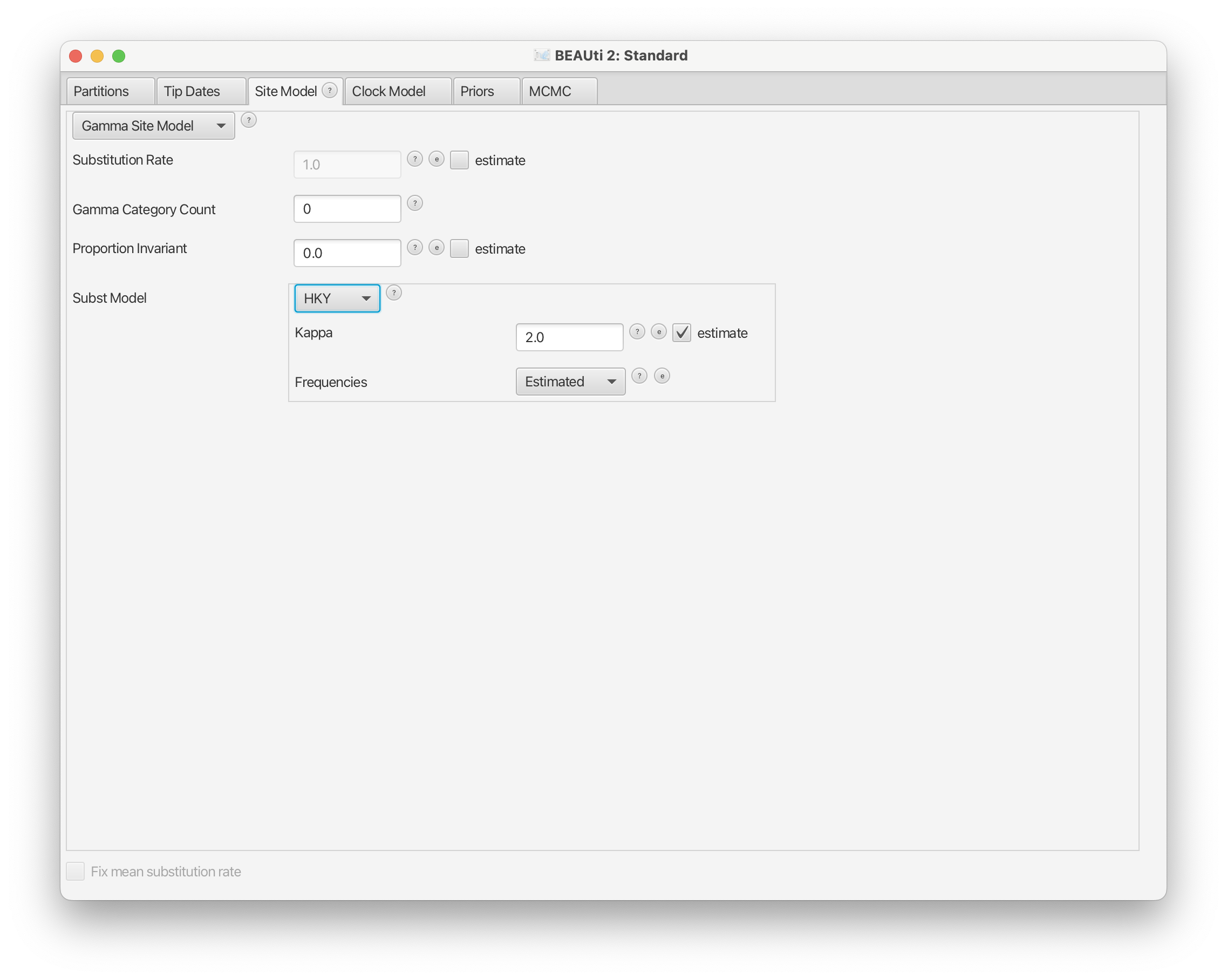
Fig. 53 : Screenshot showing how to change the substitution model in BEAUti 2.

Then, we will set the starting tree to Cluster Tree and cluster type to UPGMA in the Starting tree panel, while leaving the remaining variables to the default values. This panel is not shown by default in BEAUti 2 and requires us to click on the View --> Show Starting tree panel button.

Fig. 54 : Screenshot showing how to show the starting tree panel in BEAUti 2.

After enabling the Starting tree panel, we can set the starting tree to Cluster Tree and Cluster Type to upgma.

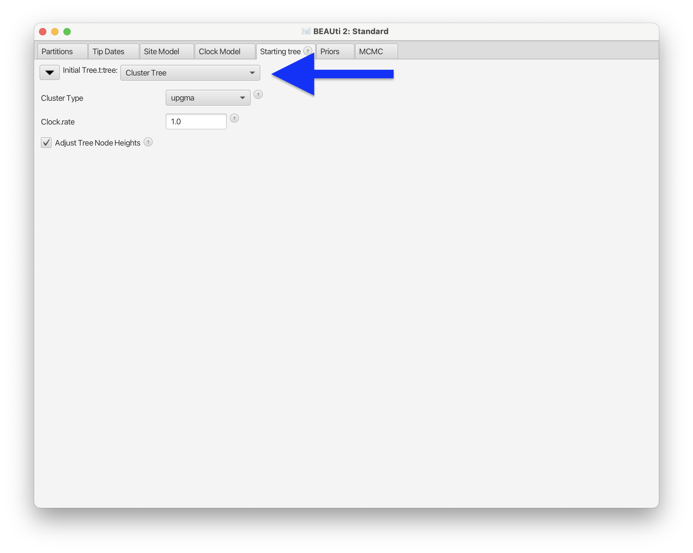
Fig. 55 : Screenshot showing how to set the starting tree to Cluster Tree and type to UPGMA in BEAUti 2.

The final setting we will change is the Chain Length in the MCMC panel, which we will set to 10^8 (add one more 0 at the end of the default value).

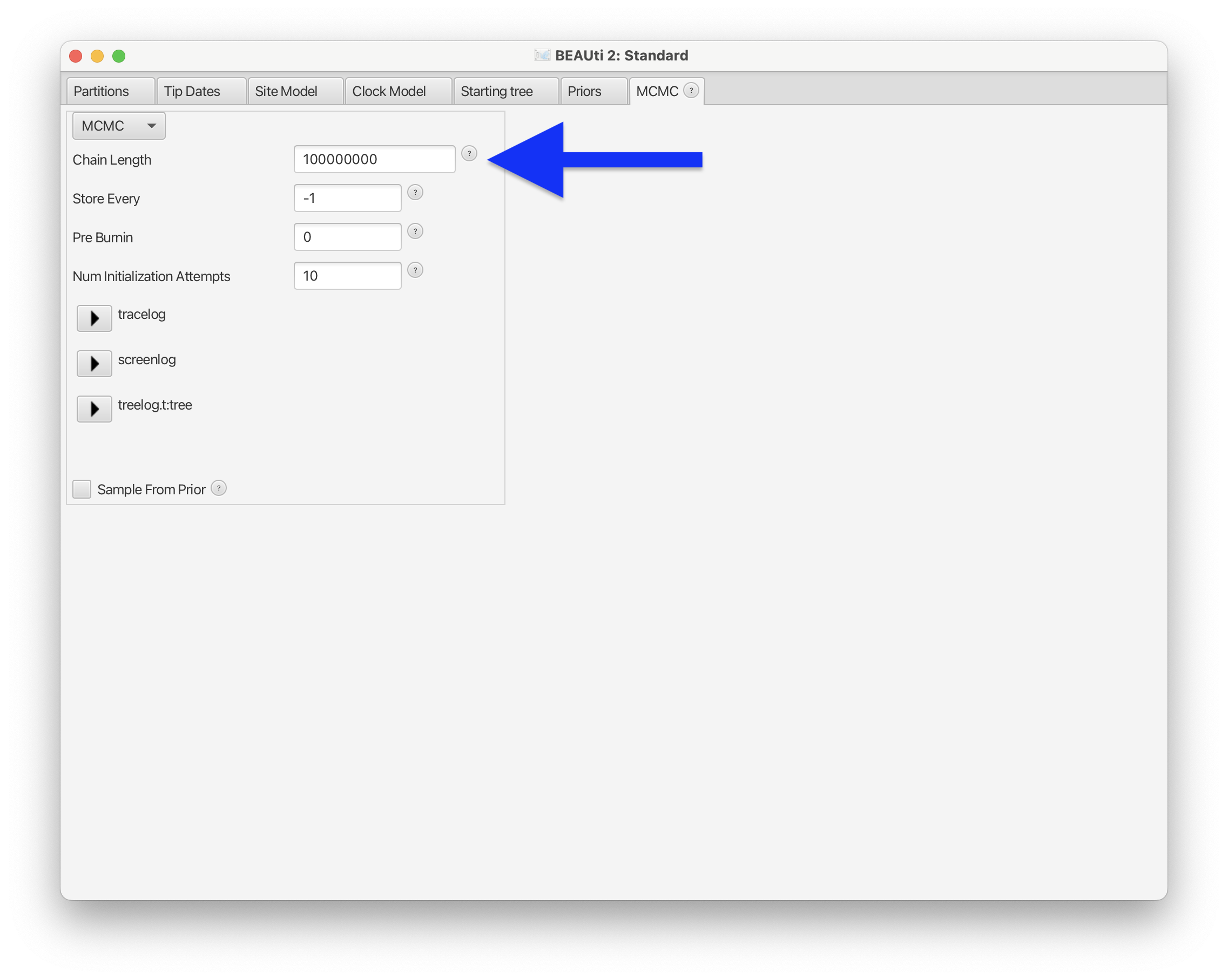
Fig. 56 : Screenshot showing how to set the chain length in BEAUti 2.

Once the Chain Length is set, we can export the data to an xml file format by pressing the File --> Save button.

Fig. 57 : Screenshot showing how to save the xml file in BEAUti 2.

For this tutorial, we will save the xml file in the 6.phylotree subdirectory and save the file as phylo_asvs.xml.

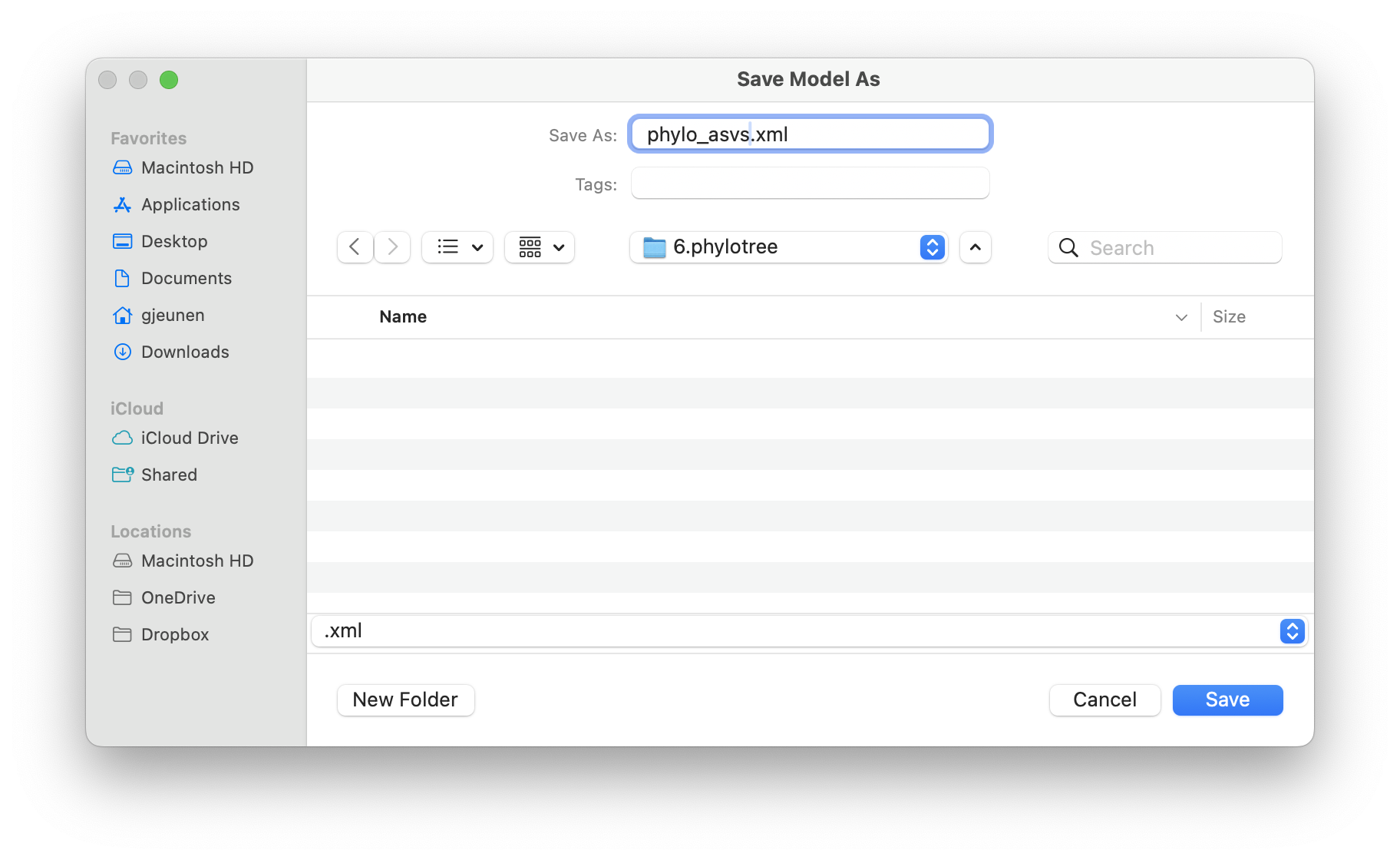
Fig. 58 : Screenshot showing the save location of the xml file for this tutorial.

4. BEAST 2

After we’ve created the xml file using BEAUti 2, we can start the BEAST 2 application.

BEAST 2 requires the xml file as Input file. We can also set the Random number seed to 2025. Finally we can set the Threads and Instances within the Run options to the maximum values of 20 for each.

Random number seed

It is important to remember and report the Random number seed to make results reproducible.

Beagle

I highly recommend installing Beagle when using BEAST 2 to generate phylogenetic trees. Creating Bayesian trees is a very computationally intensive process and can take a long time to complete (hours to days). Beagle allows BEAST to make use of the GPU cores on your system and significantly reduces computation times.

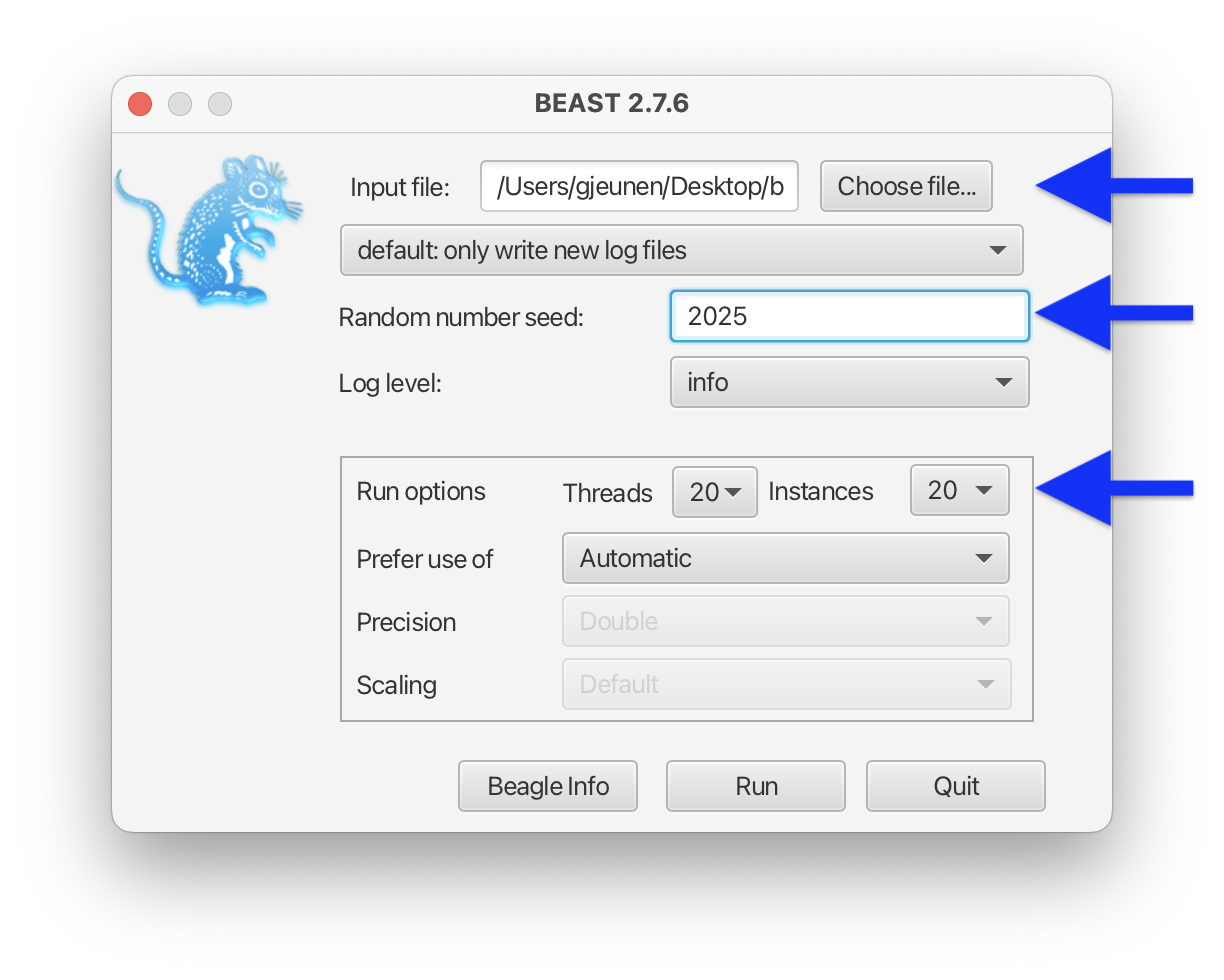
Fig. 59 : Screenshot showing the BEAST 2 settings.

Once you have set the correct settings for BEAST 2, we can start the process by pressing the Run button.

BEAST 2 output files

Since BEAST 2 will take several hours to complete for this dataset, we have provided all output files in the 6.phylotree subdirectory, including phylo_asvs.log (BEAST 2 log file to check results) and phylo_asvs-tree.trees (output trees generated by BEAST 2).

5. Tracer

After BEAST 2 completes, we can check the log file using the Tracer application. Tracer is a graphical tool for visualisation and diagnostics of MCMC (BEAST 2) output. A full explanation on the interpretation of the graphs is, unfortunately, outside the scope of this workshop. For now, we will only focus on the ESS values in the left-side panel. Ideally, they should be above 200.

After opening the Tracer application, we can click the File --> Import Trace File button.

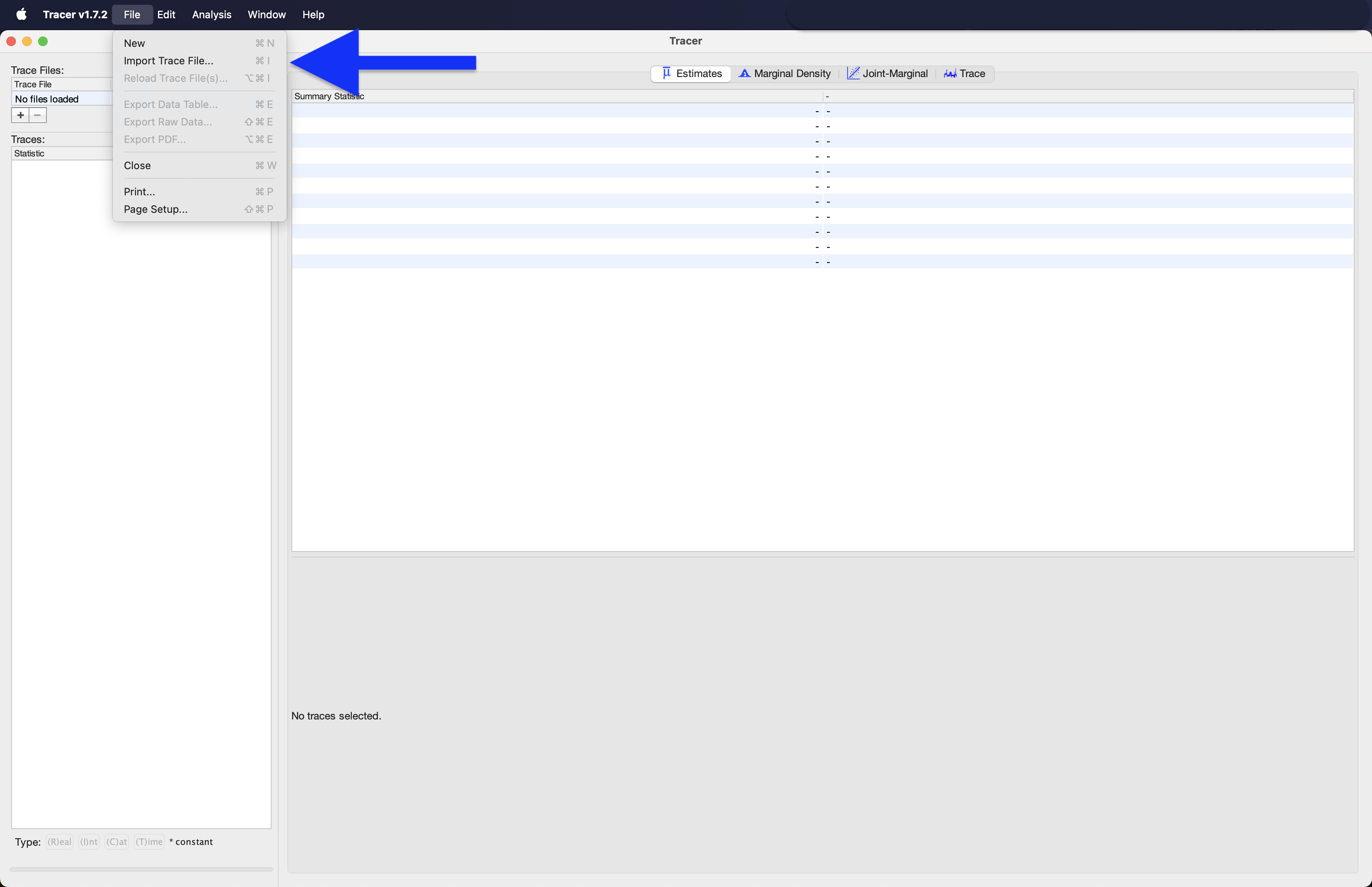
Fig. 60 : Screenshot showing the import trace file in Tracer.

We can navigate to the 6.phylotree subdirectory and select the asvs_aligned.log file.

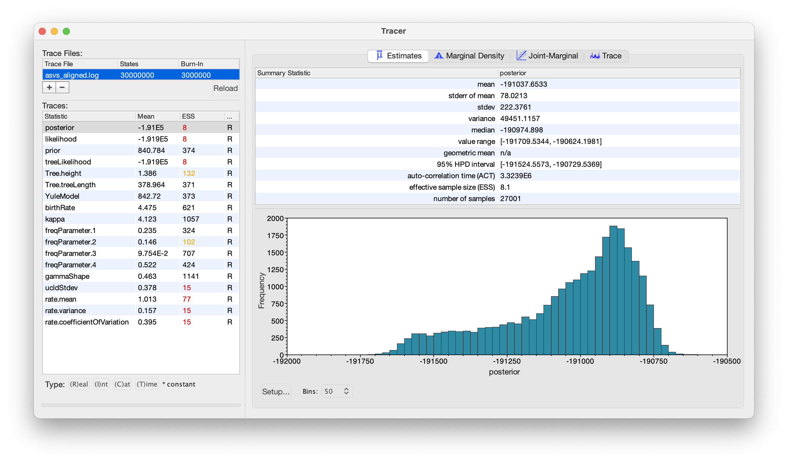
Fig. 61 : Screenshot showing the trace file results in Tracer.

From the results of the log file, we can see that multiple parameters, including very important ones such as posterior, likelihood, and treeLikelihood, have much lower ESS values than 200. Ideally, we would either run the MCMC for longer (current chain length: 3 x 10^7) or tweak some of the parameters (note: the current run took ~2 days on my laptop). We’ve included the trace file (asvs_aligned.xml.state), as well as the xml file (asvs_aligned.xml) in case you would like to optimise this tree. For the tutorial, we will go ahead with finding the best supported tree. However, please keep in mind that the tree might not be as accurate as it can be!

6. TreeAnnotator

Once we have checked the log file using Tracer, we can find the best supported tree using the TreeAnnotator application. TreeAnnotator assists in summarising the information from the sample of trees produced by BEAST 2 onto a single “target” tree. The summary information includes the posterior probabilities of the nodes in the target tree, the posterior estimates, and HPD limits of the node heights.

When opening TreeAnnotator, we will set the Node heights parameter to Mean heights, as well as select the Input Tree File, which is our asvs_aligned-tree.trees file. Finally, we will set the Output File parameter in the same folder with name asvs_aligned-tree.tree and select the Low memory option. Then, we can press the Run button.

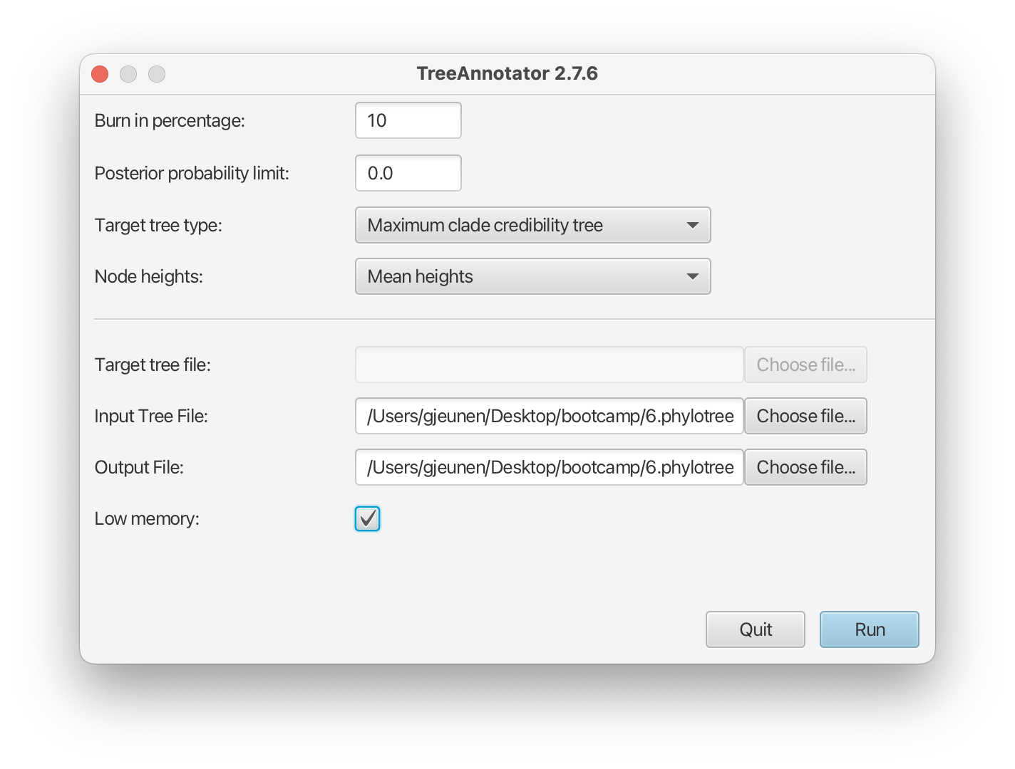
Fig. 62 : Screenshot showing the TreeAnnotator settings.

After TreeAnnotator has finished finding the best supported tree, we can close the application.

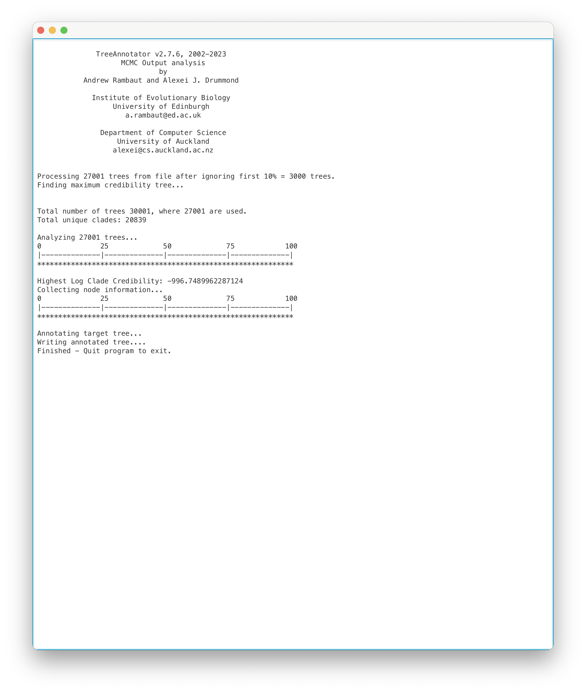
Fig. 63 : Screenshot showing the TreeAnnotator results.

7. FigTree

After exporting the best-supported tree using TreeAnnotator, we can visualise the tree quality using FigTree.

After opening the FigTree application, we can click the File --> Open button and select the asvs_aligned-tree.tree file that was generated by TreeAnnotator. Here, we can select Node Labels in the left hand-side column and set Display to posterior to determine how well branches are supported within the phylogenetic tree.

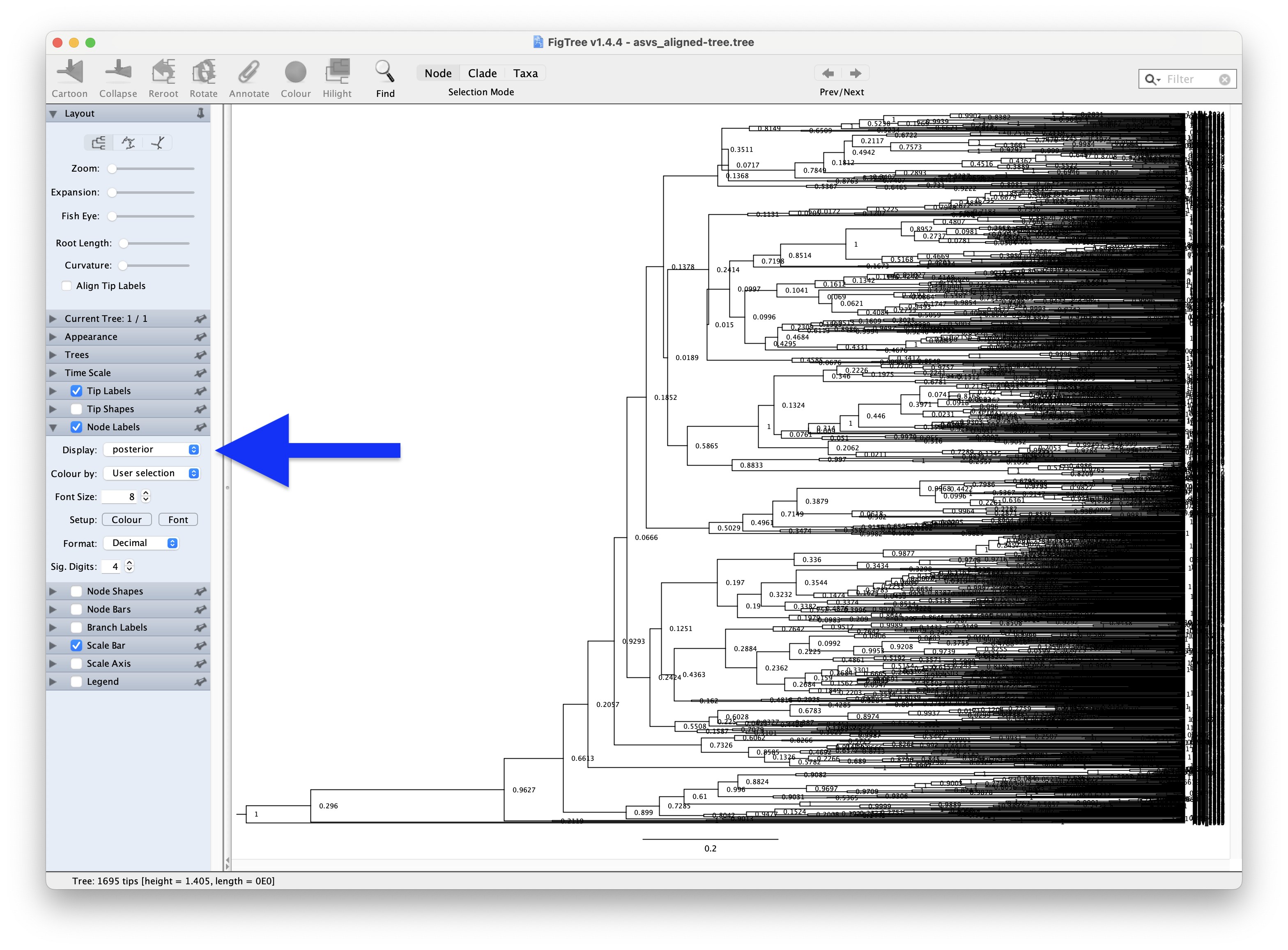
Fig. 64 : Screenshot showing the posterior values of our phylogenetic tree in FigTree.

However, given how many branches this phylogenetic tree has, it might be easier to set the Colour by parameter in Appearance to posterior.

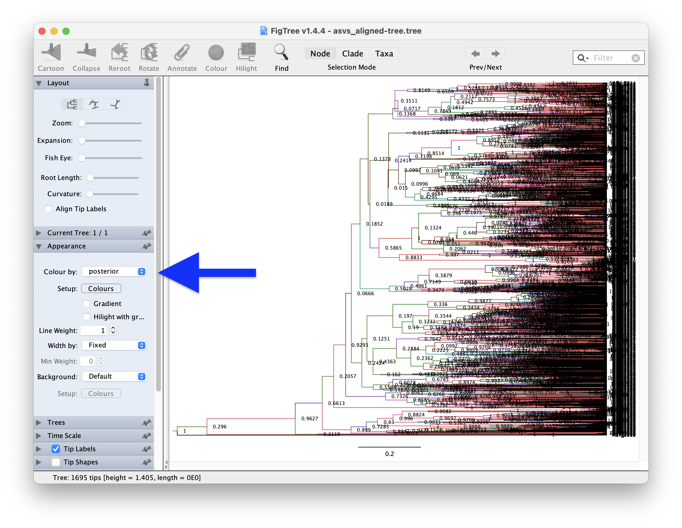
Fig. 65 : Screenshot showing the posterior values of our phylogenetic tree in branch colours in FigTree.

As expected, given the log details we explored in the Tracer application, many branches show low posterior values and are, hence, not well supported. This is something we would definitely need to fix for a scientific publication, but let’s move forward for this tutorial.

8. Visualisation in R

While the Bayesian phylogenetic tree we created enables us to explore Phylogenetic Diversity (PD) in our data (a topic we will explore during the Statistical Analysis), phylogenetic trees are also frequently included as one of the visualisations in metabarcoding publications. Today, we will show you how to generate a circular phylogenetic tree and append other data types to the phylogenetic tree. This will enable us to visualise differences in ASV detection between sample locations. The R package we will be using to generate this figure is ggtree, a fantastic R package developed by Prof. Guangchaung Yu. We will only scratch the surface of what this R package is capable of, so for more information, I recommend this book and the accompanying publication to start with.

First, let’s open a new R script and save it as phylotree_visualisation.R in the bootcamp directory. We can, then, set the working environment, load the necessary R packages, and read the data into R.

## set up the working environment
setwd(file.path(Sys.getenv("HOME"), "Desktop", "bootcamp"))
list.files()

## load necessary R packages
for (pkg in c("ape", "tidyverse", "ggtree")) {
  if (!require(pkg, character.only = TRUE)) install.packages(pkg)
  library(pkg, character.only = TRUE)
  cat(pkg, "version:", as.character(packageVersion(pkg)), "\n")
}

## read data into R
metadata <- read.table(file.path("4.results", "metadata_filtered.txt"), header = TRUE, sep = '\t', row.names = 1, check.names = FALSE, comment.char = '')
count_table <- read.table(file.path("4.results", "count_table_filtered.txt"), header = TRUE, sep = '\t', row.names = 1, check.names = FALSE, comment.char = '')
phylo_tree <- read.nexus(file.path("6.phylotree", "asvs_aligned-tree.tree"))

To plot presence-absence data per location on the phylogenetic tree, we first have to reformat the data, by grouping samples per location and transforming the data to presence-absence. Then, we have to set 0 values to NA and set 1 values to the location name. This last step is essential for creating the heatmap we will plot over the phylogenetic tree.

## reformat data
metadata <- metadata %>%
  mutate(sample = rownames(.))
count_location <- count_table %>%
  t() %>% as.data.frame() %>%
  rownames_to_column("sample") %>%
  left_join(metadata %>% select(sample, sampleLocation), by = "sample") %>%
  select(-sample) %>%
  group_by(sampleLocation) %>%
  summarise(across(everything(), sum, na.rm = TRUE)) %>%
  mutate(across(-sampleLocation, ~ if_else(.x > 0, 1, 0))) %>%
  column_to_rownames("sampleLocation") %>%
  t() %>% as.data.frame()
count_location[count_location == 0] <- NA
column_names <- names(count_location)
for (col in column_names) {
  count_location[[col]] <- ifelse(count_location[[col]] == 1, col, count_location[[col]])
}

Once we have the data formatted, we can plot the graph using the ggtree R package.

## plot tree
sample_colors <- c("Akakina" = "#EAE0DA", "Asan" = "#A0C3D2", "Ashiken" = "#E7C8C0", "Edateku" = "#B5C7A4",
                   "Gamo" = "#D4BBDD", "Heda" = "#F2D7A7", "Imaizaki" = "#A2D9D1", "Kurasaki" = "#DFA7A7", "Sakibaru" = "#C5D0E6", 
                   "Sani" = "#D9C5A0", "Taen" = "#B7D9C4", "Tatsugo" = "#E3B7D1", "Yadon" = "#A8C6D9")
circ1 <- ggtree(phylo_tree, layout = "fan", open.angle = 20, size = 0.05, color = "grey30")
circ2 <- rotate_tree(circ1, 280)
circ3 <- gheatmap(circ2, count_location, width = 0.5, offset = -0.0272,
                  color = NA, hjust = 0.5, font.size = 3, colnames = FALSE) +
  scale_fill_manual(values = sample_colors, na.value = NA) +
  theme(legend.position = "top") +
  geom_vline(xintercept = c(1.385, 1.45, 1.51, 1.575, 1.64, 1.705, 1.77,
                            1.83, 1.895, 1.955, 2.02, 2.085), linewidth = 0.1)
circ3
ggsave(filename = file.path("4.results", "phylogenetic_tree.png"), plot = circ3, bg = "white", dpi = 300) 

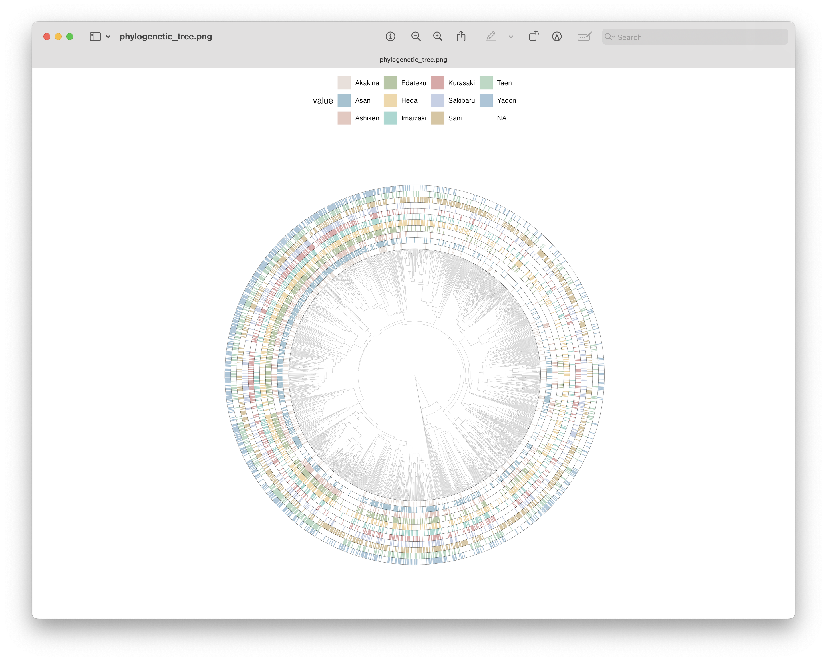
Fig. 66 : Phylogenetic tree with overlaid heatmap for ASV detection per location using the ggtree R package.

Additional customisation

Maybe try yourself to change this phylogenetic tree plot by colouring branches based on the assigned phylum. When trying, it would be best to subset the data and prune the tree to only include high confidence BLAST-hits.