Setting up the environment

1. Starting file

To follow along with this tutorial, you will need access to this website, as well as a single tarball (filename: japan_eDNA_bootcamp_files.tar.gz). The website contains all the code we will be using, while the zipped file contains all the data necessary to successfully execute the code.

To start, place the tarball (filename: japan_eDNA_bootcamp_files.tar.gz) into an empty directory you will use for this workshop. For consistency, let’s name this new folder bootcamp and place it on your Desktop.

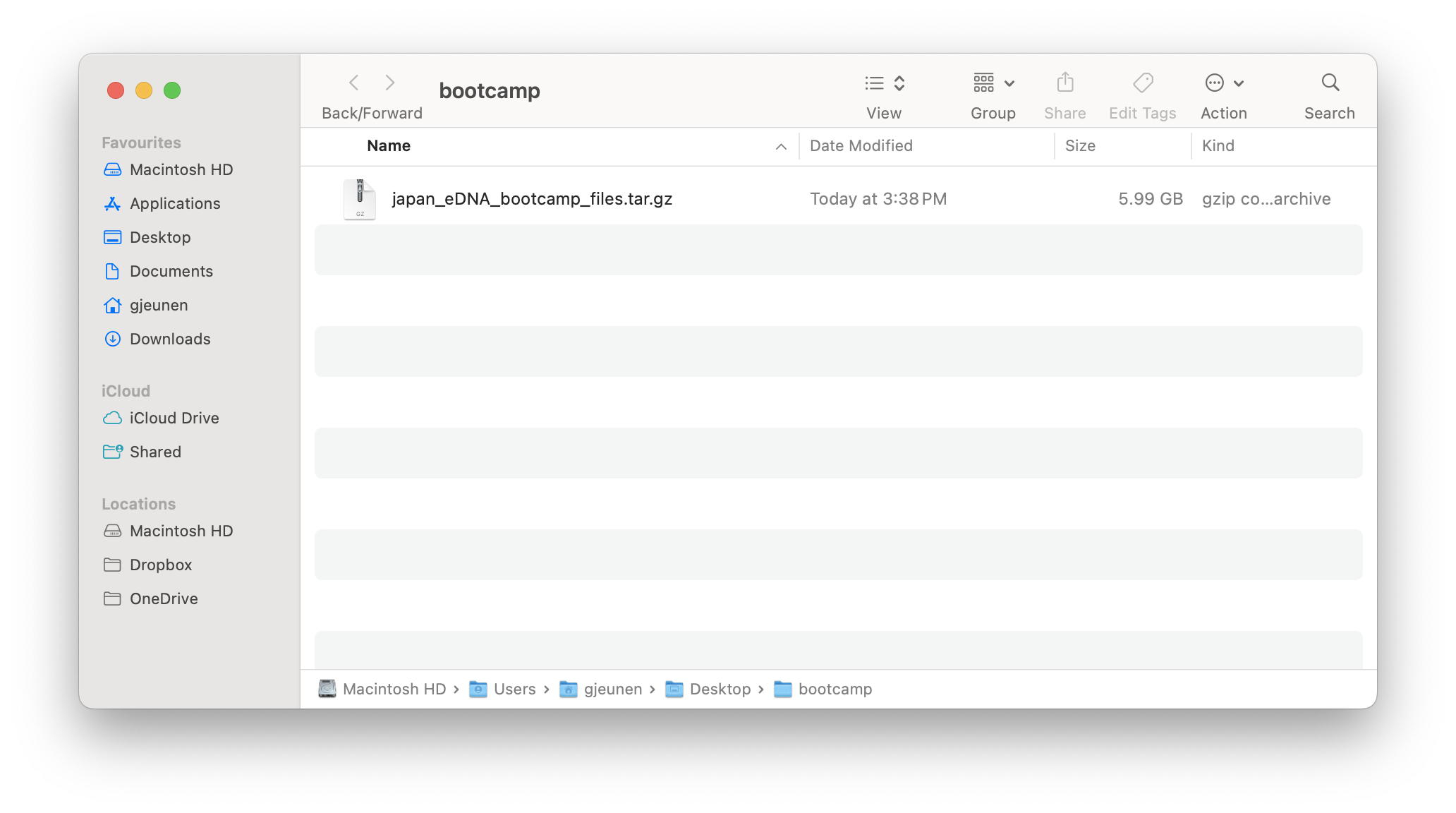
Fig. 7 : The starting screen for this workflow (note: this worflow was developed on MacOS, slight differences might be experienced on Windows or Linux)

2. RStudio

2.1 Introduction

During this course, we will be using the RStudio Desktop application, the most widely-used Integrated Development Environment (IDE) for working with R, to analyse and visualise eDNA metabarcoding data. RStudio provides a powerful and user-friendly interface for:

1. writing and executing R code

2. data wrangling

3. statistical analysis

4. publication-quality figures

5. reproducible research

While prior R experience will be beneficial, we aim to keep things simple and start with the essentials!

2.2 The RStudio interface

The RStudio interface is divided into 4 primary panels, each serving a specific purpose in data analysis. Since we will be using all of them during this bootcamp, let’s quickly introduce each of them.

1. Source Editor (Top-left)

   1. Purpose: Write, edit, and execute scripts

   2. Key features:

      1. Tabbed documents for .R scripts, notebooks, or metadata files and dataframes.

      2. Syntax highlighting for debugging.

      3. Run button to execute code line-by-line or in chunks.

2. Console and Terminal (Bottom-left)

   1. Purpose:

      1. Console: Directly interact with R to execute commands and view raw output.

      2. Terminal: Indirectly interact with the shell environment to access command-line interface (CLI) programs.

   2. Key features:

      1. > prompt for live coding.

      2. Tab-completion for functions and filenames.

      3. Up-arrow to recall previous commands.

3. Environment and History (Top-right)

   1. Environment:

      1. List all loaded objects, such as dataframes and variables

      2. Click any object to view it as a spreadsheet in the Source Editor panel.

   2. History:

      1. Review all executed commands (can be saved to a script).

4. Files, Plots, Packages, and Help (Bottom-right)

   1. Files: Navigate project directories.

   2. Plots: Visualise and export graphs as PDF/PNG for publications.

   3. Packages: Check, update, or install R packages needed for analysis.

   4. Help: Search documentation for R packages, essential for troubleshooting.

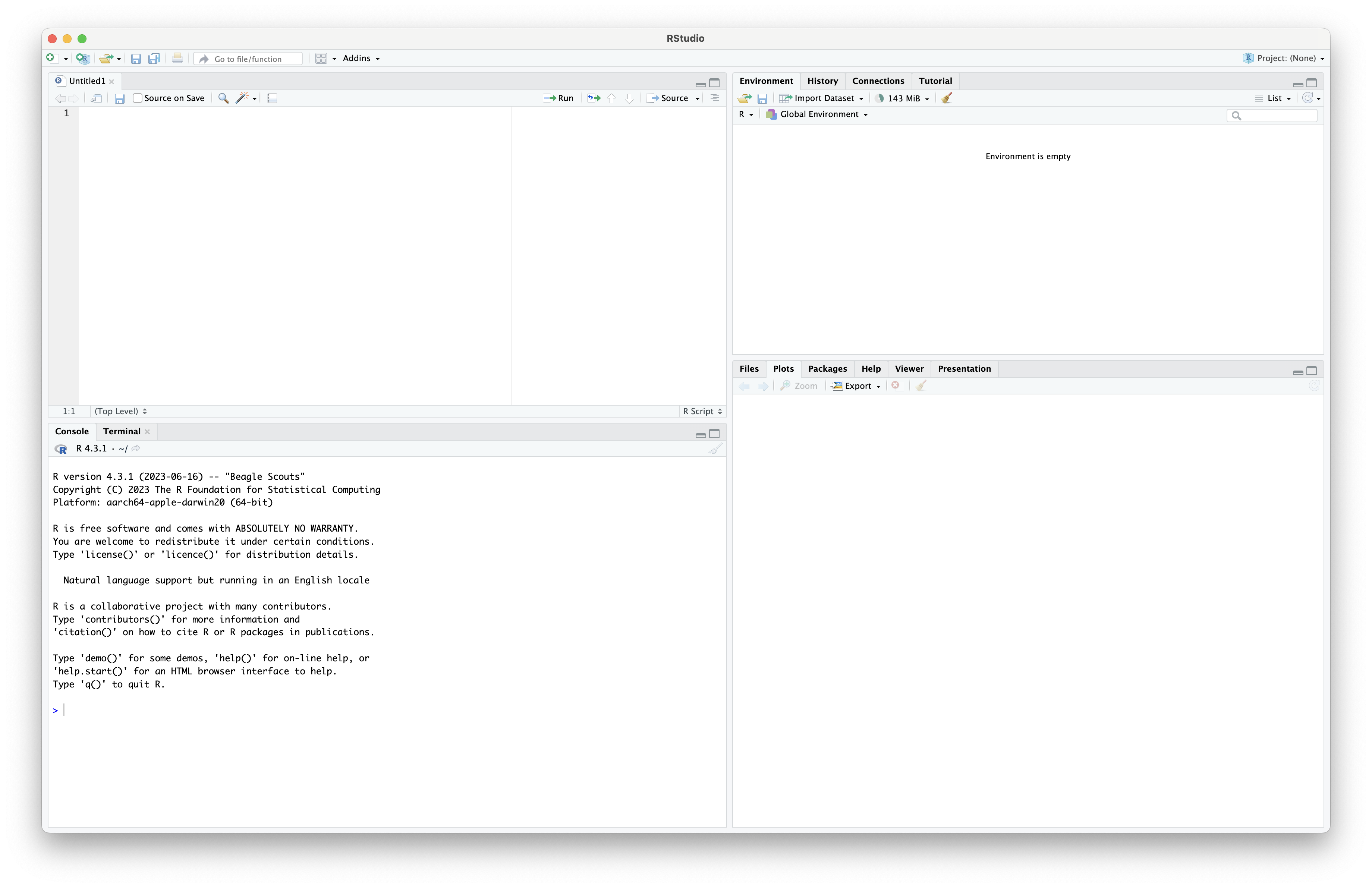
Fig. 8 : The starting screen for RStudio (note: the RStudio interface is highly customisable, so your version might look slightly different)

3. Folder structure & Starting files

3.1 Navigating and executing code in RStudio

Let’s now open RStudio and create a new R script. In this script, we will copy-paste the code from this website and execute it. To open a new R script, we can click the top-left button or press shift + command + N for MacOS and shift + ctrl + N for Windows and Linux.

Fig. 9 : Screenshot to show how to open a new R script.

The first thing we need to do is to unzip the tarball (filename: japan_eDNA_bootcamp_files.tar.gz) to gain access to all the starting files. To do this, we need to point RStudio to our newly created folder (name: bootcamp) on our Desktop. Upon starting RStudio, the current working directory is set to the home folder. We can print the current working directory by typing the following code in the R script and execute it.

getwd()

Output

> getwd()
[1] "/Users/gjeunen"

To execute the line of code, we can press the Run button on the top-right of the Source Editor screen or press command + return on MacOS or ctrl + enter on Windows and Linux. When the code is successfully executed, it will show in the Console window together with the raw output, which in this case is a string containing the information of the current working directory.

Fig. 10 : Executing our first line of R code!

Navigating to our bootcamp folder on the Desktop can be done via two different ways in RStudio. The first is via the dedicated Choose Directory... button in the Session drop down window.

Fig. 11 : Navigating between directories in RStudio using the Session dropdown window.

However, preferrable is to use the setwd() function. So, let’s use that instead for this workshop. The setwd() function usually takes in a simple string, i.e., a line of text in between quotes. However, to make the code work cross-platform, we have to provide a couple of extra bits of information, as MacOS, Linux, and Windows use different file paths.

setwd(file.path(Sys.getenv("HOME"), "Desktop", "bootcamp"))

Wen executing the getwd() function again, we will see that the path has changed to our bootcamp folder.

getwd()

Output

> getwd()
[1] "/Users/gjeunen/Desktop/bootcamp"

A final check to ensure we are in the correct folder, is to list the files within the current working directory. This should give us an output of our tarball file (filename: japan_eDNA_bootcamp_files.tar.gz).

list.files()

Output

> list.files()
[1] "japan_eDNA_bootcamp_files.tar.gz"

Now that we are in the correct folder, we can unzip the starting file to gain access to all files needed for completing the bioinformatic analysis.

untar("japan_eDNA_bootcamp_files.tar.gz")

3.2 Folder structure

Once the tarball is unzipped, we can have a look at the folder structure we will use during the workshop. For any project, it is important to organise your various files into subfolders. Throughout this course, we will be navigating between folders to run specific lines of code. It may seem confusing or tedious at first, especially as we will only be dealing with a few files during this workshop. However, remember that for many projects you can easily generate hundreds of intermediary files. So, it is best to start with good practices from the beginning.

As we did earlier, we can use the list.files() function to print all the files in the directory. We can provide the parameter include.dirs = TRUE to also print out all the subdirectories within our current working directory.

list.files(include.dirs = TRUE)

Output

> list.files(include.dirs = TRUE)
[1] "0.metadata"                       "1.raw"                            "2.trimmed"                       
[4] "3.filtered"                       "4.results"                        "5.refdb"                         
[7] "6.phylotree"                      "japan_eDNA_bootcamp_files.tar.gz"

We can see that RStudio prints the list of files and folders in columns to span the width of the Console window. However, sometimes it is easier to print results line-by-line. We can use the writeLines() function to accomplish this.

writeLines(list.files(include.dirs = TRUE))

Output

> writeLines(list.files(include.dirs = TRUE))
0.metadata
1.raw
2.trimmed
3.filtered
4.results
5.refdb
6.phylotree
japan_eDNA_bootcamp_files.tar.gz

3.3 Starting files

While most folders are currently empty, as we will populate them with files during our analysis, some folders contain the necessary starting files for the analysis. We can provide one extra parameter to the previous code, i.e., recursive = TRUE, to print out all subdirectories and files within them.

writeLines(list.files(recursive = TRUE, include.dirs = TRUE))

Output

> writeLines(list.files(recursive = TRUE, include.dirs = TRUE))
0.metadata
0.metadata/sample_metadata.txt
1.raw
1.raw/Akakina_1_S103_R1_001.fastq.gz
1.raw/Akakina_1_S103_R2_001.fastq.gz
1.raw/Akakina_2_S104_R1_001.fastq.gz
1.raw/Akakina_2_S104_R2_001.fastq.gz
1.raw/Akakina_3_S105_R1_001.fastq.gz
1.raw/Akakina_3_S105_R2_001.fastq.gz
1.raw/Asan_1_S108_R1_001.fastq.gz
1.raw/Asan_1_S108_R2_001.fastq.gz
1.raw/Asan_2_S109_R1_001.fastq.gz
1.raw/Asan_2_S109_R2_001.fastq.gz
1.raw/Asan_3_S110_R1_001.fastq.gz
1.raw/Asan_3_S110_R2_001.fastq.gz
1.raw/Ashiken_1_S124_R1_001.fastq.gz
1.raw/Ashiken_1_S124_R2_001.fastq.gz
1.raw/Ashiken_2_S125_R1_001.fastq.gz
1.raw/Ashiken_2_S125_R2_001.fastq.gz
1.raw/Ashiken_3_S126_R1_001.fastq.gz
1.raw/Ashiken_3_S126_R2_001.fastq.gz
1.raw/Edateku_1_S132_R1_001.fastq.gz
1.raw/Edateku_1_S132_R2_001.fastq.gz
1.raw/Edateku_2_S133_R1_001.fastq.gz
1.raw/Edateku_2_S133_R2_001.fastq.gz
1.raw/Edateku_3_S134_R1_001.fastq.gz
1.raw/Edateku_3_S134_R2_001.fastq.gz
1.raw/FieldControl_112122_S106_R1_001.fastq.gz
1.raw/FieldControl_112122_S106_R2_001.fastq.gz
1.raw/FieldControl_112222_S143_R1_001.fastq.gz
1.raw/FieldControl_112222_S143_R2_001.fastq.gz
1.raw/FieldControl_112422_S141_R1_001.fastq.gz
1.raw/FieldControl_112422_S141_R2_001.fastq.gz
1.raw/FilterControl_112122_S107_R1_001.fastq.gz
1.raw/FilterControl_112122_S107_R2_001.fastq.gz
1.raw/FilterControl_112222_S144_R1_001.fastq.gz
1.raw/FilterControl_112222_S144_R2_001.fastq.gz
1.raw/FilterControl_112422_S142_R1_001.fastq.gz
1.raw/FilterControl_112422_S142_R2_001.fastq.gz
1.raw/Gamo_1_S111_R1_001.fastq.gz
1.raw/Gamo_1_S111_R2_001.fastq.gz
1.raw/Gamo_2_S112_R1_001.fastq.gz
1.raw/Gamo_2_S112_R2_001.fastq.gz
1.raw/Gamo_3_S113_R1_001.fastq.gz
1.raw/Gamo_3_S113_R2_001.fastq.gz
1.raw/Heda_1_S135_R1_001.fastq.gz
1.raw/Heda_1_S135_R2_001.fastq.gz
1.raw/Heda_2_S136_R1_001.fastq.gz
1.raw/Heda_2_S136_R2_001.fastq.gz
1.raw/Heda_3_S137_R1_001.fastq.gz
1.raw/Heda_3_S137_R2_001.fastq.gz
1.raw/Imaizaki_1_S121_R1_001.fastq.gz
1.raw/Imaizaki_1_S121_R2_001.fastq.gz
1.raw/Imaizaki_2_S122_R1_001.fastq.gz
1.raw/Imaizaki_2_S122_R2_001.fastq.gz
1.raw/Imaizaki_3_S123_R1_001.fastq.gz
1.raw/Imaizaki_3_S123_R2_001.fastq.gz
1.raw/Kurasaki_1_S117_R1_001.fastq.gz
1.raw/Kurasaki_1_S117_R2_001.fastq.gz
1.raw/Kurasaki_2_S118_R1_001.fastq.gz
1.raw/Kurasaki_2_S118_R2_001.fastq.gz
1.raw/Kurasaki_3_S119_R1_001.fastq.gz
1.raw/Kurasaki_3_S119_R2_001.fastq.gz
1.raw/Sakibaru_1_S114_R1_001.fastq.gz
1.raw/Sakibaru_1_S114_R2_001.fastq.gz
1.raw/Sakibaru_2_S115_R1_001.fastq.gz
1.raw/Sakibaru_2_S115_R2_001.fastq.gz
1.raw/Sakibaru_3_S116_R1_001.fastq.gz
1.raw/Sakibaru_3_S116_R2_001.fastq.gz
1.raw/Sani_1_S97_R1_001.fastq.gz
1.raw/Sani_1_S97_R2_001.fastq.gz
1.raw/Sani_2_S98_R1_001.fastq.gz
1.raw/Sani_2_S98_R2_001.fastq.gz
1.raw/Sani_3_S99_R1_001.fastq.gz
1.raw/Sani_3_S99_R2_001.fastq.gz
1.raw/Taen_1_S129_R1_001.fastq.gz
1.raw/Taen_1_S129_R2_001.fastq.gz
1.raw/Taen_2_S130_R1_001.fastq.gz
1.raw/Taen_2_S130_R2_001.fastq.gz
1.raw/Taen_3_S131_R1_001.fastq.gz
1.raw/Taen_3_S131_R2_001.fastq.gz
1.raw/Tatsugo_1_S100_R1_001.fastq.gz
1.raw/Tatsugo_1_S100_R2_001.fastq.gz
1.raw/Tatsugo_2_S101_R1_001.fastq.gz
1.raw/Tatsugo_2_S101_R2_001.fastq.gz
1.raw/Tatsugo_3_S102_R1_001.fastq.gz
1.raw/Tatsugo_3_S102_R2_001.fastq.gz
1.raw/Yadon_1_S138_R1_001.fastq.gz
1.raw/Yadon_1_S138_R2_001.fastq.gz
1.raw/Yadon_2_S139_R1_001.fastq.gz
1.raw/Yadon_2_S139_R2_001.fastq.gz
1.raw/Yadon_3_S140_R1_001.fastq.gz
1.raw/Yadon_3_S140_R2_001.fastq.gz
2.trimmed
3.filtered
4.results
5.refdb
5.refdb/coi_blast.ndb
5.refdb/coi_blast.nhr
5.refdb/coi_blast.nin
5.refdb/coi_blast.nog
5.refdb/coi_blast.nos
5.refdb/coi_blast.not
5.refdb/coi_blast.nsq
5.refdb/coi_blast.ntf
5.refdb/coi_blast.nto
5.refdb/coi_clean.txt
5.refdb/names.dmp
5.refdb/nodes.dmp
5.refdb/nucl_gb.accession2taxid.gz
5.refdb/taxdb.btd
5.refdb/taxdb.bti
5.refdb/taxonomy4blast.sqlite3
6.phylotree
japan_eDNA_bootcamp_files.tar.gz

The output shows that we have a single sample metadata file, 90 zipped sequence files, and a formatted reference database. We will provide more details on each file in the following sections.

For now, let’s save and close the current R script. We can save it as navigation.R in the current working directory bootcamp.

Now that we have everything set up, we can get started with the bioinformatic processing of our data!