Data curation#
1. Introduction#
At this point, we have created three essential output files for eDNA metabarcoding research, including:
asvs.fasta: a fasta file containing the list and sequences of our ASVs.
count_table.txt: a tab-delimited text file containing sample IDs as columns, ASV IDs as rows, and read abundance in cells.
blast_parsed.txt: a tab-delimited text file containing the MRCA, taxonomic lineage, and BLAST values of our ASVs.
Before exploring the data and conducting the statistical analysis, however, we need to perform some data curation steps to further clean the data. Within the eDNA metabarcoding research community, there is not yet a standardised manner of data curation. However, steps that are frequently included are (list is not in order of importance):
Abundance filtering of specific detections to eliminate the risk of barcode hopping signals interfering with the analysis.
Either involves removing singleton detections or applying an abundance threshold (usually requires positive control samples).
Filtering of ASVs that have a positive detection in the negative control samples, by:
Removal of all ASVs in negative controls.
Applying an abundance threshold obtained from the read count in the negative (and positive) controls.
A statistical test.
Removal of low-confidence taxonomy assignments (if analysis is taxonomy-dependent).
Discarding samples with low read count.
Removal of PCR artefacts.
Data transformations from raw read count to relative abundance, presence-absence, or other transformations.
2. Artefact removal#
As a first data curation step, we will be removing spurious artefacts using a novel algorithm developed by our team, i.e., tombRaider. Although stringent quality filtering parameters have been employed during the bioinformatic processing steps, artefacts still persist and are known to inflate diversity estimates. These artefacts might arise from the incoproration of PCR errors (taq, the most frequently used enzyme in PCR amplification does not exhibit proofreading capabilities) or the presence of pseudogenes. For a more in depth look into artefact and artefact removel, please consult the tombRaider manuscript.
tombRaider can identify and remove artefacts using a single line of code, based on taxonomic ID, sequence similarity, the presence of stop codons, and co-occurrence patterns. For a detailed look into the workflow, please have a look at the figure below.
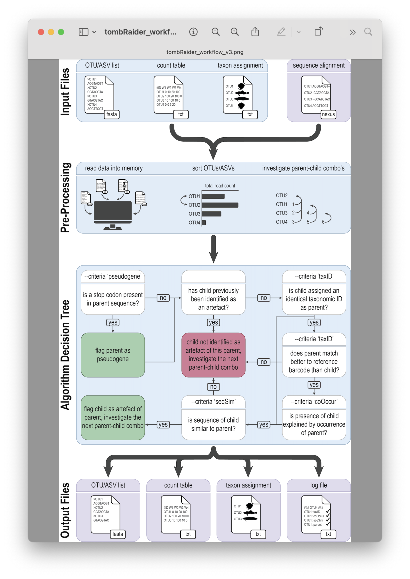
Fig. 38 : The tombRaider workflow to remove artefacts from metabarcoding data. Copyright: Jeunen et al., 2024#
Similar to CRABS, tombRaider is a CLI program written in Python. Hence, we will use the same approach as before, where we will copy-paste the code into a new text document in RStudio and execute the code in the Terminal window.
To execute tombRaider, we need to provide a list of criteria that we want to incorporate into the algorithm for deciding what is an artefact and what is not (--criteria), a count table input file (--frequency-input), a list of ASVs (--sequence-input), a file containing information on the taxonomic ID for each sequence (--taxonomy-input), the format of this file in case it is a BLAST file (--blast-format), a count table output file (--frequency-output), an output file name for the list of new ASVs (--sequence-output), a taxonomy output file name (--taxonomy-output), a log output file name (--log), the datatype to take into account (--occurrence-type), the ratio of the co-occurrence model (--occurrence-ratio), a parameter if the data needs sorting (--sort), and the sequence similarity threshold (--similarity).
So, let’s open the taxonomy_assignment.txt file and copy-paste the code below. For this tutorial, we will incorporate taxonomic ID and co-occurrence patterns into the algorithm’s decision tree to speed up the process. However, for your own data, I suggest to also include sequence similarity. One way to speed up the algorithm when including sequence similarity is to provide a multiple sequence alignment in nexus format. I suggest looking into the AlignSeqs() function of the DECIPHER R package (something we will cover when we will generate a phylogenetic tree in our dataset).
tombRaider --criteria 'taxId;coOccur' --frequency-input count_table.txt --sequence-input asvs.fasta --taxonomy-input blast_results.txt --blast-format '6 qaccver saccver staxid sscinames length pident mismatch qcovs evalue bitscore qstart qend sstart send gapopen' --frequency-output count_table_new.txt --sequence-output asvs_new.fasta --taxonomy-output blast_results_new.txt --log tombraider_log.txt --occurrence-type abundance --occurrence-ratio 'count;1' --sort 'total read count'
Output
/// tombRaider | v1.0
| Included Criteria | taxid, cooccur
| Excluded Criteria | pseudogene, seqsim
| Reading Files | ━━━━━━━━━━━━━━━━━━━━━━━━━━━━━━━━━━━━━━━━ 100% 0:00:00 0:00:00
| Identify artefacts | ━━━━━━━━━━━━━━━━━━━━━━━━━━━━━━━━━━━━━━━━ 100% 0:00:00 0:00:26
| Summary Statistics |
| Total # of ASVs | 8314
|Total # of Artefacts | 5585 (67.18%)
| Artefact List |
| parent: ASV_1 | children: ASV_17, ASV_745, ASV_5227, ASV_6080, ASV_8249, ASV_8247, ASV_7370, ASV_7325, ASV_7660, ASV_8306, ASV_7307
| parent: ASV_2 | children: ASV_4, ASV_12, ASV_13, ASV_18, ASV_20, ASV_27, ASV_32, ASV_42, ASV_43, ASV_48, ASV_62, ASV_68, ASV_76, ASV_84, ASV_91, ASV_131, ASV_133, ASV_141, ASV_147,
ASV_155, ASV_264, ASV_282, ASV_805, ASV_1168, ASV_1245, ASV_1529, ASV_2160, ASV_3646, ASV_3702, ASV_3862, ASV_4452, ASV_7373, ASV_7371, ASV_8305, ASV_8296
| parent: ASV_3 | children: ASV_47, ASV_52, ASV_97, ASV_136, ASV_140, ASV_148, ASV_151, ASV_161, ASV_176, ASV_255, ASV_349, ASV_442, ASV_473, ASV_492, ASV_620, ASV_650, ASV_694,
ASV_730, ASV_744, ASV_784, ASV_843, ASV_995, ASV_1400, ASV_1462, ASV_1603, ASV_1720, ASV_1813, ASV_2149, ASV_2419, ASV_3023, ASV_3204, ASV_4883, ASV_7863, ASV_7251, ASV_4009, ASV_8037, ASV_8086
| parent: ASV_5 | children: ASV_40, ASV_239, ASV_275, ASV_549, ASV_590, ASV_946, ASV_1126, ASV_1471, ASV_2255, ASV_2812, ASV_4365, ASV_7039, ASV_7096, ASV_6913, ASV_6316, ASV_7292,
ASV_7473, ASV_8302, ASV_4505, ASV_4234, ASV_4745, ASV_5465, ASV_7400, ASV_5533, ASV_6841, ASV_7885, ASV_8138
| parent: ASV_6 | children: ASV_16, ASV_23, ASV_73, ASV_101, ASV_143, ASV_171, ASV_179, ASV_190, ASV_266, ASV_267, ASV_334, ASV_339, ASV_345, ASV_371, ASV_424, ASV_466, ASV_478,
ASV_583, ASV_603, ASV_631, ASV_698, ASV_715, ASV_865, ASV_896, ASV_910, ASV_938, ASV_957, ASV_1034, ASV_1059, ASV_1112, ASV_1105, ASV_1132, ASV_1134, ASV_1280, ASV_1330, ASV_1387, ASV_1510,
ASV_1557, ASV_1624, ASV_1697, ASV_1696, ASV_1769, ASV_1770, ASV_1827, ASV_1999, ASV_2000, ASV_2225, ASV_2434, ASV_2435, ASV_2945, ASV_3133, ASV_3940, ASV_3867, ASV_3865, ASV_4653
| parent: ASV_8 | children: ASV_61, ASV_65, ASV_2290, ASV_2499, ASV_3092, ASV_4944
| parent: ASV_9 | children: ASV_125, ASV_168, ASV_328, ASV_1271, ASV_1548, ASV_1906, ASV_3594, ASV_3984, ASV_4449
| parent: ASV_10 | children: ASV_735, ASV_4217, ASV_4372, ASV_4949, ASV_5774, ASV_5658, ASV_5598, ASV_6633
| parent: ASV_11 | children: ASV_594, ASV_776, ASV_815
| parent: ASV_14 | children: ASV_38, ASV_173, ASV_450, ASV_625, ASV_807, ASV_945, ASV_1304, ASV_1589, ASV_1960, ASV_2668, ASV_3200, ASV_3619, ASV_4474, ASV_5973, ASV_5390, ASV_7604,
ASV_7689
| parent: ASV_15 | children: ASV_104, ASV_6645
| parent: ASV_19 | children: ASV_298, ASV_7535
| parent: ASV_21 | children: ASV_386, ASV_685, ASV_714, ASV_740, ASV_962, ASV_1538
| parent: ASV_22 | child: ASV_428
| parent: ASV_24 | children: ASV_167, ASV_5025, ASV_8192
| parent: ASV_26 | child: ASV_70
| parent: ASV_28 | children: ASV_268, ASV_821, ASV_2359, ASV_7385, ASV_3181
| parent: ASV_29 | children: ASV_755, ASV_2712, ASV_3123, ASV_6547
| parent: ASV_30 | children: ASV_154, ASV_258, ASV_359, ASV_534, ASV_635, ASV_690, ASV_832, ASV_1009, ASV_1450, ASV_1475, ASV_1645, ASV_1776, ASV_1806, ASV_2436, ASV_2550, ASV_2768,
ASV_2817, ASV_2831, ASV_2977, ASV_3146, ASV_3197, ASV_3428, ASV_3840, ASV_3678, ASV_3903, ASV_4572, ASV_4384, ASV_4997, ASV_5141, ASV_5368, ASV_5237, ASV_5557, ASV_7063, ASV_7067, ASV_6067,
ASV_6031, ASV_6090, ASV_7217, ASV_7184, ASV_7625, ASV_4647, ASV_3093, ASV_4882, ASV_4902, ASV_5476, ASV_6745, ASV_5897, ASV_2347, ASV_6104, ASV_4052, ASV_3853, ASV_4112, ASV_5037, ASV_6541,
ASV_7198, ASV_8286, ASV_4523, ASV_7254, ASV_4875, ASV_6925, ASV_7145, ASV_7746, ASV_6401
| parent: ASV_31 | children: ASV_74, ASV_85, ASV_110, ASV_204, ASV_314, ASV_361, ASV_365, ASV_380, ASV_435, ASV_486, ASV_591, ASV_675, ASV_757, ASV_830, ASV_831, ASV_833, ASV_886,
ASV_1165, ASV_1247, ASV_1518, ASV_1607, ASV_1836, ASV_1963, ASV_2021, ASV_2018, ASV_2050, ASV_2178, ASV_2696, ASV_2651, ASV_3151, ASV_4632, ASV_5070, ASV_4739, ASV_4696, ASV_5322, ASV_5323,
ASV_7021, ASV_6175, ASV_6131, ASV_6512, ASV_8155, ASV_7253, ASV_7191, ASV_7443, ASV_7477, ASV_7503, ASV_8300, ASV_8299
| parent: ASV_33 | children: ASV_174, ASV_209, ASV_289, ASV_304, ASV_358, ASV_392, ASV_403, ASV_539, ASV_558, ASV_584, ASV_663, ASV_748, ASV_794, ASV_806, ASV_885, ASV_895, ASV_916,
ASV_1005, ASV_1033, ASV_1032, ASV_1062, ASV_1080, ASV_1082, ASV_1139, ASV_1150, ASV_1149, ASV_1143, ASV_1170, ASV_1186, ASV_1238, ASV_1267, ASV_1277, ASV_1276, ASV_1298, ASV_1326, ASV_1366,
ASV_1365, ASV_1403, ASV_1424, ASV_1431, ASV_1433, ASV_1429, ASV_1447, ASV_1499, ASV_1571, ASV_1598, ASV_1656, ASV_1654, ASV_1653, ASV_1674, ASV_1672, ASV_1683, ASV_1754, ASV_1771, ASV_1750,
ASV_1749, ASV_1743, ASV_1792, ASV_1787, ASV_1817, ASV_1826, ASV_1841, ASV_1844, ASV_1895, ASV_1891, ASV_1892, ASV_1897, ASV_1907, ASV_1932, ASV_1981, ASV_1979, ASV_1976, ASV_2037, ASV_2073,
ASV_2119, ASV_2125, ASV_2099, ASV_2101, ASV_2172, ASV_2173, ASV_2152, ASV_2214, ASV_2216, ASV_2228, ASV_2199, ASV_2198, ASV_2279, ASV_2289, ASV_2247, ASV_2261, ASV_2260, ASV_2248, ASV_2339,
ASV_2351, ASV_2352, ASV_2329, ASV_2331, ASV_2328, ASV_2319, ASV_2318, ASV_2414, ASV_2412, ASV_2403, ASV_2404, ASV_2438, ASV_2399, ASV_2423, ASV_2417, ASV_2365, ASV_2397, ASV_2396, ASV_2394,
ASV_2497, ASV_2487, ASV_2482, ASV_2517, ASV_2515, ASV_2514, ASV_2506, ASV_2503, ASV_2480, ASV_2439, ASV_2468, ASV_2470, ASV_2582, ASV_2581, ASV_2579, ASV_2616, ASV_2597, ASV_2617, ASV_2570,
ASV_2536, ASV_2525, ASV_2524, ASV_2558, ASV_2559, ASV_2556, ASV_2555, ASV_2680, ASV_2676, ASV_2671, ASV_2672, ASV_2669, ASV_2694, ASV_2633, ASV_2632, ASV_2640, ASV_2770, ASV_2814, ASV_2805,
ASV_2800, ASV_2797, ASV_2761, ASV_2732, ASV_2748, ASV_2749, ASV_2740, ASV_2739, ASV_2737, ASV_2909, ASV_2891, ASV_2925, ASV_2889, ASV_2942, ASV_2933, ASV_2890, ASV_2845, ASV_2849, ASV_2834,
ASV_2832, ASV_2877, ASV_2872, ASV_2857, ASV_2858, ASV_3067, ASV_3079, ASV_3084, ASV_3064, ASV_3086, ASV_3051, ASV_3052, ASV_3053, ASV_3063, ASV_3087, ASV_3116, ASV_3125, ASV_3126, ASV_3109,
ASV_3095, ASV_3096, ASV_3097, ASV_3099, ASV_3031, ASV_3043, ASV_2987, ASV_2989, ASV_2993, ASV_3042, ASV_2963, ASV_3034, ASV_3039, ASV_3041, ASV_3032, ASV_3004, ASV_3267, ASV_3266, ASV_3260,
ASV_3262, ASV_3238, ASV_3311, ASV_3312, ASV_3319, ASV_3231, ASV_3328, ASV_3329, ASV_3331, ASV_3286, ASV_3287, ASV_3232, ASV_3161, ASV_3167, ASV_3131, ASV_3180, ASV_3207, ASV_3208, ASV_3209,
ASV_3206, ASV_3217, ASV_3183, ASV_3184, ASV_3182, ASV_3185, ASV_3186, ASV_3202, ASV_3195, ASV_3196, ASV_3508, ASV_3489, ASV_3488, ASV_3464, ASV_3465, ASV_3474, ASV_3485, ASV_3486, ASV_3570,
ASV_3557, ASV_3562, ASV_3579, ASV_3580, ASV_3523, ASV_3526, ASV_3534, ASV_3536, ASV_3541, ASV_3547, ASV_3456, ASV_3373, ASV_3384, ASV_3358, ASV_3394, ASV_3430, ASV_3432, ASV_3446, ASV_3453,
ASV_3401, ASV_3402, ASV_3405, ASV_3407, ASV_3418, ASV_3421, ASV_3412, ASV_3769, ASV_3767, ASV_3777, ASV_3722, ASV_3738, ASV_3741, ASV_3838, ASV_3842, ASV_3843, ASV_3720, ASV_3855, ASV_3803,
ASV_3810, ASV_3811, ASV_3814, ASV_3818, ASV_3820, ASV_3721, ASV_3749, ASV_3719, ASV_3630, ASV_3629, ASV_3628, ASV_3623, ASV_3633, ASV_3643, ASV_3602, ASV_3694, ASV_3695, ASV_3688, ASV_3708,
ASV_3709, ASV_3686, ASV_3662, ASV_3661, ASV_3676, ASV_3681, ASV_3671, ASV_4096, ASV_4125, ASV_4054, ASV_4061, ASV_4057, ASV_4079, ASV_4077, ASV_4068, ASV_4066, ASV_4198, ASV_4196, ASV_4193,
ASV_4192, ASV_4190, ASV_4185, ASV_4203, ASV_4179, ASV_4223, ASV_4222, ASV_4220, ASV_4219, ASV_4215, ASV_4213, ASV_4210, ASV_4180, ASV_4155, ASV_4152, ASV_4139, ASV_4137, ASV_4154, ASV_4157,
ASV_4164, ASV_4162, ASV_3918, ASV_3917, ASV_3915, ASV_3948, ASV_3941, ASV_3937, ASV_3879, ASV_3893, ASV_3890, ASV_4008, ASV_4000, ASV_4019, ASV_4020, ASV_4036, ASV_4034, ASV_4033, ASV_4021,
ASV_3960, ASV_3959, ASV_3973, ASV_3988, ASV_3983, ASV_3979, ASV_3978, ASV_3974, ASV_4506, ASV_4509, ASV_4488, ASV_4527, ASV_4524, ASV_4522, ASV_4521, ASV_4517, ASV_4458, ASV_4457, ASV_4441,
ASV_4440, ASV_4482, ASV_4481, ASV_4477, ASV_4462, ASV_4471, ASV_4466, ASV_4463, ASV_4539, ASV_4605, ASV_4604, ASV_4621, ASV_4634, ASV_4643, ASV_4642, ASV_4637, ASV_4627, ASV_4624, ASV_4559,
ASV_4552, ASV_4567, ASV_4579, ASV_4433, ASV_4299, ASV_4297, ASV_4315, ASV_4314, ASV_4313, ASV_4312, ASV_4244, ASV_4243, ASV_4236, ASV_4432, ASV_4249, ASV_4259, ASV_4255, ASV_4406, ASV_4431,
ASV_4427, ASV_4423, ASV_4418, ASV_4382, ASV_4354, ASV_4353, ASV_4349, ASV_4339, ASV_4338, ASV_4333, ASV_4355, ASV_4374, ASV_4367, ASV_4362, ASV_5028, ASV_5034, ASV_5008, ASV_5040, ASV_5014,
ASV_5015, ASV_5039, ASV_5041, ASV_5042, ASV_5058, ASV_5051, ASV_5052, ASV_4959, ASV_4952, ASV_4953, ASV_4958, ASV_4937, ASV_4938, ASV_4943, ASV_4945, ASV_4947, ASV_4993, ASV_4971, ASV_4974,
ASV_4976, ASV_4978, ASV_4985, ASV_4981, ASV_4983, ASV_4984, ASV_5176, ASV_5170, ASV_5175, ASV_5168, ASV_5169, ASV_5154, ASV_5162, ASV_5213, ASV_5208, ASV_5212, ASV_5205, ASV_5216, ASV_5206,
ASV_5204, ASV_5190, ASV_5192, ASV_5193, ASV_5196, ASV_5149, ASV_5098, ASV_5099, ASV_5100, ASV_5103, ASV_5105, ASV_5096, ASV_5106, ASV_5095, ASV_5086, ASV_5080, ASV_5084, ASV_5134, ASV_5118,
ASV_5129, ASV_4743, ASV_4721, ASV_4727, ASV_4728, ASV_4750, ASV_4751, ASV_4760, ASV_4755, ASV_4758, ASV_4759, ASV_4761, ASV_4762, ASV_4668, ASV_4659, ASV_4931, ASV_4676, ASV_4704, ASV_4712,
ASV_4698, ASV_4685, ASV_4886, ASV_4891, ASV_4879, ASV_4896, ASV_4920, ASV_4898, ASV_4900, ASV_4901, ASV_4907, ASV_4909, ASV_4811, ASV_4812, ASV_4814, ASV_4815, ASV_4793, ASV_4804, ASV_4799,
ASV_4803, ASV_4802, ASV_4825, ASV_4834, ASV_4831, ASV_4836, ASV_5758, ASV_5753, ASV_5760, ASV_5730, ASV_5803, ASV_5777, ASV_5818, ASV_5802, ASV_5782, ASV_5783, ASV_5797, ASV_5655, ASV_5650,
ASV_5654, ASV_5659, ASV_5666, ASV_5667, ASV_5670, ASV_5626, ASV_5628, ASV_5631, ASV_5633, ASV_5640, ASV_5645, ASV_5700, ASV_5702, ASV_5703, ASV_5705, ASV_5707, ASV_5708, ASV_5709, ASV_5710,
ASV_5711, ASV_5680, ASV_5682, ASV_5683, ASV_5685, ASV_5687, ASV_5688, ASV_5689, ASV_5694, ASV_5695, ASV_5965, ASV_5968, ASV_5975, ASV_5952, ASV_5930, ASV_5937, ASV_5942, ASV_5948, ASV_5949,
ASV_5979, ASV_6005, ASV_6007, ASV_6013, ASV_6024, ASV_6025, ASV_5624, ASV_6006, ASV_6000, ASV_5854, ASV_5858, ASV_5926, ASV_5868, ASV_5869, ASV_5874, ASV_5853, ASV_5833, ASV_5834, ASV_5838,
ASV_5839, ASV_5848, ASV_5907, ASV_5908, ASV_5913, ASV_5920, ASV_5922, ASV_5924, ASV_5925, ASV_5904, ASV_5880, ASV_5890, ASV_5891, ASV_5893, ASV_5352, ASV_5355, ASV_5358, ASV_5359, ASV_5362,
ASV_5344, ASV_5327, ASV_5331, ASV_5332, ASV_5339, ASV_5342, ASV_5371, ASV_5402, ASV_5409, ASV_5410, ASV_5417, ASV_5396, ASV_5373, ASV_5374, ASV_5376, ASV_5379, ASV_5388, ASV_5389, ASV_5254,
ASV_5263, ASV_5243, ASV_5222, ASV_5226, ASV_5231, ASV_5232, ASV_5304, ASV_5308, ASV_5309, ASV_5311, ASV_5312, ASV_5295, ASV_5292, ASV_5274, ASV_5280, ASV_5281, ASV_5284, ASV_5422, ASV_5550,
ASV_5551, ASV_5552, ASV_5554, ASV_5556, ASV_5559, ASV_5567, ASV_5568, ASV_5549, ASV_5528, ASV_5529, ASV_5540, ASV_5544, ASV_5574, ASV_5609, ASV_5575, ASV_5580, ASV_5587, ASV_5594, ASV_5595,
ASV_5462, ASV_5464, ASV_5466, ASV_5471, ASV_5433, ASV_5427, ASV_5430, ASV_5446, ASV_5438, ASV_5442, ASV_5445, ASV_5443, ASV_5499, ASV_5507, ASV_5512, ASV_5513, ASV_5515, ASV_5518, ASV_5519,
ASV_5496, ASV_5480, ASV_5478, ASV_5489, ASV_6748, ASV_6747, ASV_6749, ASV_6756, ASV_6760, ASV_6761, ASV_6762, ASV_6763, ASV_6764, ASV_6703, ASV_6706, ASV_6709, ASV_6710, ASV_6712, ASV_6717,
ASV_6719, ASV_6720, ASV_6721, ASV_6726, ASV_6765, ASV_6814, ASV_6820, ASV_6823, ASV_6768, ASV_6775, ASV_6776, ASV_6796, ASV_6612, ASV_6613, ASV_6614, ASV_6598, ASV_6619, ASV_6620, ASV_6622,
ASV_6624, ASV_6626, ASV_6627, ASV_6628, ASV_6629, ASV_6597, ASV_6580, ASV_6834, ASV_6573, ASV_6579, ASV_6596, ASV_6591, ASV_6592, ASV_6671, ASV_6674, ASV_6678, ASV_6684, ASV_6685, ASV_6666,
ASV_6636, ASV_6642, ASV_6644, ASV_6646, ASV_6658, ASV_6660, ASV_6662, ASV_6663, ASV_6835, ASV_7020, ASV_7008, ASV_7011, ASV_7013, ASV_7022, ASV_7023, ASV_7025, ASV_7027, ASV_7032, ASV_6970,
ASV_6972, ASV_6983, ASV_7088, ASV_7077, ASV_7078, ASV_7079, ASV_7087, ASV_7089, ASV_7090, ASV_7102, ASV_7072, ASV_7041, ASV_7042, ASV_7057, ASV_6969, ASV_6873, ASV_6874, ASV_6876, ASV_6877,
ASV_6878, ASV_6889, ASV_6890, ASV_6891, ASV_6893, ASV_6900, ASV_6851, ASV_6863, ASV_6864, ASV_6866, ASV_6951, ASV_6904, ASV_6954, ASV_6956, ASV_6958, ASV_6960, ASV_6962, ASV_6963, ASV_6965,
ASV_6934, ASV_6905, ASV_6923, ASV_6927, ASV_6928, ASV_6929, ASV_6198, ASV_6202, ASV_6213, ASV_6218, ASV_6221, ASV_6222, ASV_6176, ASV_6177, ASV_6182, ASV_6227, ASV_6278, ASV_6275, ASV_6276,
ASV_6279, ASV_6283, ASV_6293, ASV_6261, ASV_6238, ASV_6241, ASV_6252, ASV_6253, ASV_6254, ASV_6255, ASV_6256, ASV_6257, ASV_6258, ASV_6295, ASV_6074, ASV_6063, ASV_6072, ASV_6079, ASV_6081,
ASV_6083, ASV_6088, ASV_6059, ASV_6028, ASV_6034, ASV_6036, ASV_6037, ASV_6039, ASV_6044, ASV_6048, ASV_6049, ASV_6050, ASV_6129, ASV_6130, ASV_6135, ASV_6144, ASV_6152, ASV_6153, ASV_6155,
ASV_6123, ASV_6096, ASV_6098, ASV_6099, ASV_6102, ASV_6110, ASV_6111, ASV_6122, ASV_6294, ASV_6471, ASV_6483, ASV_6487, ASV_6488, ASV_6442, ASV_6449, ASV_6451, ASV_6452, ASV_6453, ASV_6459,
ASV_6498, ASV_6535, ASV_6536, ASV_6540, ASV_6542, ASV_6550, ASV_6551, ASV_6553, ASV_6556, ASV_6533, ASV_6507, ASV_6508, ASV_6514, ASV_6515, ASV_6527, ASV_6346, ASV_6336, ASV_6337, ASV_6338,
ASV_6342, ASV_6343, ASV_6347, ASV_6351, ASV_6360, ASV_6303, ASV_6306, ASV_6307, ASV_6322, ASV_6323, ASV_6362, ASV_6364, ASV_6405, ASV_6406, ASV_6407, ASV_6410, ASV_6422, ASV_6423, ASV_6397,
ASV_6366, ASV_6375, ASV_6376, ASV_6377, ASV_6387, ASV_6388, ASV_7896, ASV_7889, ASV_7898, ASV_7911, ASV_7901, ASV_7916, ASV_7853, ASV_7850, ASV_7848, ASV_7879, ASV_7872, ASV_7865, ASV_7919,
ASV_7959, ASV_7975, ASV_7985, ASV_7990, ASV_7988, ASV_7983, ASV_7981, ASV_7933, ASV_7928, ASV_7926, ASV_7923, ASV_7950, ASV_7748, ASV_7763, ASV_7757, ASV_7734, ASV_7710, ASV_7705, ASV_7701,
ASV_7698, ASV_7992, ASV_7730, ASV_7728, ASV_7725, ASV_7720, ASV_7719, ASV_7824, ASV_7820, ASV_7812, ASV_7825, ASV_7836, ASV_7834, ASV_7833, ASV_7832, ASV_7807, ASV_7783, ASV_7782, ASV_7781,
ASV_7778, ASV_7774, ASV_7773, ASV_7788, ASV_7803, ASV_7802, ASV_7800, ASV_7798, ASV_7797, ASV_7796, ASV_7793, ASV_7993, ASV_8194, ASV_8186, ASV_8183, ASV_8181, ASV_8197, ASV_8198, ASV_8213,
ASV_8211, ASV_8203, ASV_8177, ASV_8146, ASV_8145, ASV_8161, ASV_8165, ASV_8162, ASV_8253, ASV_8267, ASV_7696, ASV_8270, ASV_8285, ASV_8276, ASV_8275, ASV_8232, ASV_8230, ASV_8225, ASV_8223,
ASV_8222, ASV_8219, ASV_8233, ASV_8244, ASV_8248, ASV_8242, ASV_8030, ASV_8045, ASV_8041, ASV_8038, ASV_8033, ASV_8032, ASV_7996, ASV_8012, ASV_8027, ASV_8023, ASV_8022, ASV_8018, ASV_8104,
ASV_8117, ASV_8113, ASV_8111, ASV_8132, ASV_8135, ASV_8068, ASV_8079, ASV_8084, ASV_8098, ASV_7300, ASV_7297, ASV_7295, ASV_7294, ASV_7293, ASV_7303, ASV_7397, ASV_7319, ASV_7316, ASV_7308,
ASV_7287, ASV_7286, ASV_7264, ASV_7262, ASV_7261, ASV_7259, ASV_7256, ASV_7322, ASV_7366, ASV_7365, ASV_7394, ASV_7393, ASV_7390, ASV_7388, ASV_7381, ASV_7384, ASV_7359, ASV_7337, ASV_7332,
ASV_7342, ASV_7343, ASV_7348, ASV_7346, ASV_7154, ASV_7152, ASV_7149, ASV_7147, ASV_7146, ASV_7143, ASV_7169, ASV_7158, ASV_7164, ASV_7162, ASV_7137, ASV_7136, ASV_7116, ASV_7113, ASV_7112,
ASV_7108, ASV_7104, ASV_7103, ASV_7119, ASV_7247, ASV_7225, ASV_7245, ASV_7243, ASV_7242, ASV_7239, ASV_7238, ASV_7190, ASV_7189, ASV_7186, ASV_7183, ASV_7192, ASV_7207, ASV_7196, ASV_7619,
ASV_7613, ASV_7609, ASV_7608, ASV_7584, ASV_7583, ASV_7563, ASV_7551, ASV_7578, ASV_7577, ASV_7574, ASV_7573, ASV_7572, ASV_7571, ASV_7568, ASV_7621, ASV_7675, ASV_7666, ASV_7677, ASV_7687,
ASV_7634, ASV_7633, ASV_7650, ASV_7649, ASV_7648, ASV_7646, ASV_7645, ASV_7452, ASV_7450, ASV_7447, ASV_7444, ASV_7437, ASV_7453, ASV_7455, ASV_7470, ASV_7469, ASV_7466, ASV_7463, ASV_7412,
ASV_7432, ASV_7431, ASV_7430, ASV_7429, ASV_7428, ASV_7525, ASV_7524, ASV_7523, ASV_7474, ASV_7521, ASV_7520, ASV_7517, ASV_7542, ASV_7540, ASV_7539, ASV_7530, ASV_7534, ASV_7532, ASV_7509,
ASV_7491, ASV_7489, ASV_7481, ASV_7479, ASV_7478, ASV_7505, ASV_7496, ASV_8303, ASV_8307, ASV_8314
| parent: ASV_34 | children: ASV_375, ASV_494, ASV_595, ASV_684, ASV_902, ASV_942, ASV_1325, ASV_3666, ASV_3962, ASV_6245
| parent: ASV_35 | children: ASV_377, ASV_481, ASV_646, ASV_917, ASV_968, ASV_1179, ASV_1339, ASV_1496, ASV_1856, ASV_1839, ASV_1925, ASV_1964, ASV_2001, ASV_2162, ASV_2267, ASV_2239,
ASV_2349, ASV_2379, ASV_2519, ASV_2510, ASV_2472, ASV_2618, ASV_2645, ASV_2947, ASV_2966, ASV_3011, ASV_3017, ASV_3248, ASV_3543, ASV_3634, ASV_4056, ASV_4545, ASV_4429, ASV_5030, ASV_4988,
ASV_4706, ASV_4869, ASV_4807, ASV_4797, ASV_5602, ASV_6742, ASV_7091, ASV_7064, ASV_6046, ASV_6545, ASV_6511, ASV_6411, ASV_7947, ASV_7940, ASV_8156, ASV_8258, ASV_8228, ASV_7317, ASV_7340,
ASV_7326, ASV_7150, ASV_7174, ASV_7110, ASV_7220, ASV_7188, ASV_7399, ASV_7570, ASV_7693, ASV_7548, ASV_2950, ASV_3137, ASV_4530, ASV_6848, ASV_4941, ASV_4250
| parent: ASV_36 | children: ASV_145, ASV_3370, ASV_8088
| parent: ASV_39 | child: ASV_132
| parent: ASV_41 | children: ASV_83, ASV_89, ASV_105, ASV_220, ASV_227, ASV_290, ASV_331, ASV_350, ASV_367, ASV_463, ASV_619, ASV_770, ASV_918, ASV_949, ASV_979, ASV_1136, ASV_1318,
ASV_1626, ASV_2176, ASV_2179, ASV_3888, ASV_4292, ASV_4320, ASV_6735, ASV_6655, ASV_7007, ASV_2723, ASV_5167, ASV_6368, ASV_7260, ASV_2307, ASV_2486, ASV_5019, ASV_7131, ASV_7970
| parent: ASV_44 | children: ASV_116, ASV_228, ASV_252, ASV_269, ASV_313, ASV_318, ASV_383, ASV_422, ASV_429, ASV_469, ASV_513, ASV_518, ASV_585, ASV_653, ASV_689, ASV_710, ASV_716,
ASV_721, ASV_742, ASV_754, ASV_785, ASV_841, ASV_874, ASV_875, ASV_879, ASV_921, ASV_933, ASV_939, ASV_953, ASV_955, ASV_965, ASV_978, ASV_984, ASV_987, ASV_992, ASV_997, ASV_1015, ASV_1038,
ASV_1050, ASV_1057, ASV_1073, ASV_1088, ASV_1119, ASV_1130, ASV_1142, ASV_1162, ASV_1208, ASV_1209, ASV_1225, ASV_1231, ASV_1248, ASV_1244, ASV_1266, ASV_1264, ASV_1296, ASV_1324, ASV_1335,
ASV_1333, ASV_1348, ASV_1350, ASV_1381, ASV_1380, ASV_1397, ASV_1390, ASV_1391, ASV_1422, ASV_1432, ASV_1461, ASV_1489, ASV_1474, ASV_1501, ASV_1528, ASV_1527, ASV_1546, ASV_1577, ASV_1556,
ASV_1588, ASV_1610, ASV_1638, ASV_1630, ASV_1625, ASV_1640, ASV_1647, ASV_1692, ASV_1710, ASV_1700, ASV_1725, ASV_1716, ASV_1713, ASV_1752, ASV_1793, ASV_1788, ASV_1819, ASV_1821, ASV_1801,
ASV_1865, ASV_1831, ASV_1847, ASV_1876, ASV_1942, ASV_1947, ASV_1933, ASV_1918, ASV_1910, ASV_1914, ASV_1917, ASV_1921, ASV_1924, ASV_1926, ASV_1927, ASV_1989, ASV_1965, ASV_1958, ASV_1974,
ASV_2038, ASV_2008, ASV_2054, ASV_2046, ASV_2122, ASV_2129, ASV_2108, ASV_2106, ASV_2157, ASV_2161, ASV_2154, ASV_2139, ASV_2150, ASV_2203, ASV_2177, ASV_2183, ASV_2275, ASV_2282, ASV_2264,
ASV_2293, ASV_2283, ASV_2265, ASV_2299, ASV_2300, ASV_2312, ASV_2325, ASV_2323, ASV_2415, ASV_2411, ASV_2407, ASV_2405, ASV_2428, ASV_2380, ASV_2491, ASV_2501, ASV_2485, ASV_2478, ASV_2444,
ASV_2442, ASV_2467, ASV_2587, ASV_2578, ASV_2596, ASV_2595, ASV_2604, ASV_2540, ASV_2539, ASV_2531, ASV_2530, ASV_2562, ASV_2674, ASV_2693, ASV_2625, ASV_2623, ASV_2660, ASV_2649, ASV_2783,
ASV_2786, ASV_2776, ASV_2794, ASV_2731, ASV_2716, ASV_2718, ASV_2921, ASV_2908, ASV_2828, ASV_2882, ASV_2884, ASV_3115, ASV_2983, ASV_2984, ASV_2973, ASV_3022, ASV_3162, ASV_3173, ASV_3152,
ASV_3134, ASV_3141, ASV_3210, ASV_3501, ASV_3506, ASV_3558, ASV_3525, ASV_3376, ASV_3380, ASV_3338, ASV_3339, ASV_3344, ASV_3345, ASV_3454, ASV_3615, ASV_3592, ASV_3604, ASV_3607, ASV_3650,
ASV_3679, ASV_4080, ASV_4042, ASV_3909, ASV_3873, ASV_3870, ASV_3885, ASV_4003, ASV_4032, ASV_3994, ASV_3967, ASV_3989, ASV_4490, ASV_4296, ASV_4231, ASV_4228, ASV_4225, ASV_4252, ASV_4713,
ASV_4686, ASV_5262, ASV_5241, ASV_5590
| parent: ASV_45 | children: ASV_183, ASV_234, ASV_288, ASV_568, ASV_1954, ASV_2166, ASV_3007, ASV_4023, ASV_4827, ASV_5534, ASV_6771, ASV_7014, ASV_7036, ASV_6056, ASV_6496, ASV_6348,
ASV_7873, ASV_8082, ASV_7594, ASV_7663, ASV_2141, ASV_2190, ASV_2699, ASV_2995, ASV_4641, ASV_4843, ASV_5732, ASV_6641, ASV_6998, ASV_7971, ASV_7815, ASV_7811, ASV_7601, ASV_7624, ASV_7683,
ASV_3263
| parent: ASV_46 | children: ASV_139, ASV_311, ASV_1795, ASV_1864, ASV_2208, ASV_2589, ASV_2906, ASV_3752, ASV_4358, ASV_4970, ASV_7699
| parent: ASV_49 | children: ASV_1124, ASV_1896, ASV_8304
| parent: ASV_51 | child: ASV_3439
| parent: ASV_53 | children: ASV_4278, ASV_7963
| parent: ASV_54 | children: ASV_412, ASV_517, ASV_658, ASV_8040, ASV_3008, ASV_3176, ASV_4592, ASV_5458, ASV_5473, ASV_6944, ASV_6445
| parent: ASV_55 | children: ASV_1079, ASV_1825, ASV_2202, ASV_2286, ASV_5264, ASV_6053, ASV_6379, ASV_3667, ASV_6466
| parent: ASV_56 | children: ASV_187, ASV_540, ASV_1010, ASV_5627, ASV_6974, ASV_985, ASV_1051, ASV_3044, ASV_4202, ASV_5865, ASV_3276, ASV_5085, ASV_5809, ASV_6875, ASV_6858, ASV_6394,
ASV_5944, ASV_7336, ASV_8044
| parent: ASV_57 | children: ASV_859, ASV_1288
| parent: ASV_58 | child: ASV_1658
| parent: ASV_60 | children: ASV_656, ASV_851, ASV_1590, ASV_2568, ASV_3913, ASV_4789, ASV_4913, ASV_5945, ASV_7603, ASV_7556
| parent: ASV_63 | children: ASV_92, ASV_94, ASV_130, ASV_1506, ASV_1727, ASV_2334, ASV_3736, ASV_6443, ASV_6120
| parent: ASV_66 | child: ASV_4113
| parent: ASV_67 | children: ASV_1018, ASV_1646, ASV_3425
| parent: ASV_69 | children: ASV_389, ASV_395, ASV_399, ASV_438, ASV_461, ASV_643, ASV_713, ASV_731, ASV_870, ASV_969, ASV_1890, ASV_2656, ASV_2894, ASV_3159, ASV_3462, ASV_3663,
ASV_4370, ASV_4769, ASV_4710, ASV_5364, ASV_5297, ASV_7075, ASV_7065, ASV_6943, ASV_6233, ASV_7944, ASV_8196, ASV_7304, ASV_7626, ASV_7647, ASV_5076, ASV_5808, ASV_5679, ASV_6187, ASV_8226,
ASV_8061, ASV_7672, ASV_3325, ASV_3907, ASV_4377, ASV_4876, ASV_4821, ASV_6793, ASV_7752, ASV_7659, ASV_8166
| parent: ASV_72 | children: ASV_436, ASV_1026, ASV_1127, ASV_1128, ASV_1189, ASV_1338, ASV_1615, ASV_1961, ASV_2209, ASV_2276, ASV_2653, ASV_2997, ASV_3352, ASV_3395, ASV_3596,
ASV_4575, ASV_4310, ASV_4254, ASV_5138, ASV_5131, ASV_5696, ASV_5548, ASV_5485, ASV_6996, ASV_6879, ASV_6448, ASV_6381, ASV_7912, ASV_7726, ASV_7128, ASV_7175, ASV_7231, ASV_1031, ASV_6854,
ASV_4648, ASV_7244
| parent: ASV_75 | children: ASV_543, ASV_1874, ASV_3498, ASV_5163, ASV_5570, ASV_8298
| parent: ASV_78 | children: ASV_216, ASV_520, ASV_529, ASV_575, ASV_608, ASV_762, ASV_823, ASV_842, ASV_928, ASV_996, ASV_1036, ASV_1053, ASV_1173, ASV_1182, ASV_1200, ASV_1237,
ASV_1242, ASV_1251, ASV_1263, ASV_1293, ASV_1321, ASV_1359, ASV_1417, ASV_1525, ASV_1568, ASV_1584, ASV_1820, ASV_1959, ASV_2044, ASV_2091, ASV_2234, ASV_2233, ASV_2311, ASV_2324, ASV_2369,
ASV_2447, ASV_2572, ASV_2566, ASV_2637, ASV_2720, ASV_2860, ASV_2868, ASV_3046, ASV_3283, ASV_3247, ASV_3253, ASV_3201, ASV_3469, ASV_3850, ASV_3637, ASV_4218, ASV_3968, ASV_3965, ASV_4629,
ASV_4626, ASV_4325, ASV_4238, ASV_5181, ASV_5199, ASV_4927, ASV_4791, ASV_5962, ASV_6021, ASV_5350, ASV_5381, ASV_5230, ASV_5520, ASV_6215, ASV_6164, ASV_6101, ASV_6115, ASV_6546, ASV_6522,
ASV_6525, ASV_6302, ASV_8264, ASV_8220, ASV_7375, ASV_7391, ASV_7362, ASV_7156, ASV_7193, ASV_7398, ASV_7559, ASV_6263, ASV_6136, ASV_5681
| parent: ASV_80 | children: ASV_397, ASV_729, ASV_2074, ASV_2549, ASV_4028, ASV_4375, ASV_5144, ASV_5333, ASV_6829, ASV_6204, ASV_7335, ASV_7355, ASV_7685
| parent: ASV_81 | child: ASV_1679
| parent: ASV_88 | child: ASV_4544
| parent: ASV_90 | children: ASV_2820, ASV_5835, ASV_5223, ASV_6815
| parent: ASV_93 | children: ASV_327, ASV_641
| parent: ASV_95 | child: ASV_8312
| parent: ASV_96 | children: ASV_743, ASV_915, ASV_976, ASV_1118, ASV_1377, ASV_1535, ASV_1583, ASV_1711, ASV_1887, ASV_2032, ASV_2513, ASV_2575, ASV_2754, ASV_3410, ASV_3830, ASV_3655,
ASV_4233, ASV_5007, ASV_5183, ASV_5729, ASV_6171, ASV_6084, ASV_6089, ASV_6380, ASV_7960, ASV_8251, ASV_7483, ASV_2062, ASV_3971, ASV_4480, ASV_6001, ASV_6128, ASV_8119, ASV_5436
| parent: ASV_98 | children: ASV_432, ASV_553, ASV_630, ASV_699, ASV_1137, ASV_1191, ASV_1748, ASV_2577, ASV_3258, ASV_3533, ASV_3732, ASV_4260, ASV_4689, ASV_5343, ASV_7537
| parent: ASV_99 | children: ASV_1334, ASV_3153, ASV_3480, ASV_5810, ASV_7001
| parent: ASV_100 | children: ASV_4476, ASV_6937
| parent: ASV_102 | children: ASV_409, ASV_455, ASV_508, ASV_626, ASV_640, ASV_956, ASV_4153, ASV_5239, ASV_5511
| parent: ASV_106 | children: ASV_551, ASV_954, ASV_1437, ASV_1594, ASV_1673, ASV_3019, ASV_6219
| parent: ASV_107 | children: ASV_325, ASV_366, ASV_391, ASV_465, ASV_809, ASV_967, ASV_1023, ASV_1041, ASV_1097, ASV_1212, ASV_1476, ASV_1805, ASV_2273, ASV_2389, ASV_2460, ASV_2612,
ASV_2677, ASV_3057, ASV_5980, ASV_5989, ASV_5269, ASV_8107, ASV_3871, ASV_7142, ASV_1774, ASV_3718, ASV_4723, ASV_4652, ASV_5314, ASV_6064, ASV_8174, ASV_8005, ASV_3868, ASV_4491, ASV_6912,
ASV_7157, ASV_7219, ASV_4420, ASV_6567, ASV_6653
| parent: ASV_109 | children: ASV_1473, ASV_2392
| parent: ASV_112 | children: ASV_242, ASV_531, ASV_1544, ASV_1593, ASV_1777, ASV_2020, ASV_2061, ASV_2249, ASV_2469, ASV_2537, ASV_2647, ASV_3494, ASV_3699, ASV_4183, ASV_3921, ASV_5672,
ASV_5452, ASV_5463, ASV_5425, ASV_6196, ASV_6186, ASV_6189, ASV_6244, ASV_6157, ASV_6468, ASV_6464, ASV_8112, ASV_8128, ASV_7288, ASV_7378, ASV_7422
| parent: ASV_114 | children: ASV_421, ASV_597, ASV_667, ASV_904, ASV_1113, ASV_1616, ASV_1634, ASV_2238, ASV_2237, ASV_2650, ASV_2846, ASV_3404, ASV_4270, ASV_7345, ASV_8311, ASV_3148,
ASV_4899, ASV_5649, ASV_5306, ASV_6119
| parent: ASV_117 | child: ASV_7664
| parent: ASV_118 | children: ASV_280, ASV_677, ASV_1103, ASV_2212, ASV_5819, ASV_7617, ASV_7654
| parent: ASV_119 | children: ASV_360, ASV_394, ASV_1466, ASV_2542
| parent: ASV_123 | children: ASV_1098, ASV_1465, ASV_2069, ASV_3567, ASV_5123, ASV_5765, ASV_5927, ASV_7010, ASV_6973, ASV_3846, ASV_4300, ASV_7279
| parent: ASV_127 | children: ASV_347, ASV_538, ASV_541, ASV_711, ASV_1203, ASV_1609, ASV_1677, ASV_1703, ASV_1722, ASV_1842, ASV_1969, ASV_2026, ASV_2067, ASV_2111, ASV_2335, ASV_2337,
ASV_2358, ASV_2422, ASV_2489, ASV_2454, ASV_2567, ASV_2551, ASV_2662, ASV_2715, ASV_2855, ASV_3158, ASV_3130, ASV_3216, ASV_3382, ASV_3724, ASV_3802, ASV_3816, ASV_4148, ASV_4511, ASV_4485,
ASV_4598, ASV_4323, ASV_4957, ASV_5092, ASV_4872, ASV_5856, ASV_5850, ASV_5919, ASV_5256, ASV_5268, ASV_5271, ASV_5289, ASV_5612, ASV_7050, ASV_6837, ASV_6163, ASV_6042, ASV_6052, ASV_6296,
ASV_6426, ASV_7987, ASV_7935, ASV_8208, ASV_7596, ASV_7591, ASV_7632, ASV_7401, ASV_1786, ASV_2400, ASV_3519, ASV_6862, ASV_4992, ASV_4855
| parent: ASV_135 | child: ASV_3774
| parent: ASV_137 | children: ASV_500, ASV_525, ASV_950, ASV_1020, ASV_1099, ASV_1166, ASV_1273, ASV_1456, ASV_2356, ASV_3156, ASV_3483, ASV_5016, ASV_5120, ASV_6593, ASV_7598, ASV_7692
| parent: ASV_138 | children: ASV_413, ASV_430, ASV_490, ASV_647, ASV_679, ASV_827, ASV_834, ASV_926, ASV_1213, ASV_1511, ASV_1627, ASV_1886, ASV_2257, ASV_2630, ASV_4324, ASV_4306,
ASV_5299, ASV_856, ASV_1312, ASV_1483, ASV_1759, ASV_2118, ASV_2406, ASV_3316, ASV_3139, ASV_3340, ASV_4123, ASV_4478, ASV_4601, ASV_4330, ASV_5044, ASV_5186, ASV_5117, ASV_5641, ASV_5983,
ASV_5370, ASV_5260, ASV_5541, ASV_6959, ASV_6931, ASV_6132, ASV_7712, ASV_8217, ASV_7277, ASV_7351, ASV_4161, ASV_7070, ASV_8284, ASV_6358, ASV_6108, ASV_8056
| parent: ASV_142 | children: ASV_300, ASV_822, ASV_993, ASV_1157, ASV_906, ASV_3860
| parent: ASV_144 | child: ASV_838
| parent: ASV_146 | children: ASV_511, ASV_555, ASV_836, ASV_3639, ASV_4048, ASV_3883
| parent: ASV_150 | children: ASV_1232, ASV_1736, ASV_5122, ASV_8102
| parent: ASV_152 | child: ASV_1047
| parent: ASV_156 | children: ASV_2827, ASV_4763, ASV_5912
| parent: ASV_157 | children: ASV_2362, ASV_4445, ASV_7515
| parent: ASV_158 | children: ASV_1239, ASV_1302, ASV_1707
| parent: ASV_159 | children: ASV_905, ASV_1069, ASV_1145, ASV_1425, ASV_2965, ASV_4513, ASV_6543, ASV_8301, ASV_8293, ASV_8292
| parent: ASV_160 | child: ASV_504
| parent: ASV_162 | children: ASV_2045, ASV_3226, ASV_3503, ASV_3995, ASV_5276, ASV_5455, ASV_6839
| parent: ASV_163 | children: ASV_1565, ASV_1714, ASV_2534, ASV_2543, ASV_2932, ASV_4131, ASV_4158, ASV_5158, ASV_5137, ASV_4912, ASV_5735, ASV_5569, ASV_5498, ASV_6794, ASV_7767,
ASV_8004, ASV_7392, ASV_6600
| parent: ASV_164 | children: ASV_519, ASV_1169, ASV_3755, ASV_5486, ASV_7854, ASV_2481
| parent: ASV_165 | children: ASV_574, ASV_881, ASV_927, ASV_977, ASV_975, ASV_1427, ASV_1641, ASV_1731, ASV_1872, ASV_1919, ASV_2016, ASV_2251, ASV_2313, ASV_3233, ASV_3553, ASV_3847,
ASV_4039, ASV_3895, ASV_3894, ASV_5150, ASV_4665, ASV_4666, ASV_5964, ASV_5321, ASV_7015, ASV_6932, ASV_6264, ASV_6273, ASV_6274, ASV_6231, ASV_6057, ASV_6093, ASV_7627, ASV_7560, ASV_7487,
ASV_4709, ASV_6429, ASV_8235, ASV_8110
| parent: ASV_169 | children: ASV_402, ASV_817, ASV_1655, ASV_2097, ASV_2253, ASV_5382, ASV_7034, ASV_8289
| parent: ASV_170 | children: ASV_857, ASV_868, ASV_1206, ASV_2593, ASV_2756, ASV_3593, ASV_5005, ASV_5348, ASV_5488, ASV_8101, ASV_8097, ASV_1379, ASV_1881, ASV_5050, ASV_6378, ASV_8236,
ASV_4189, ASV_5112, ASV_4778, ASV_5845, ASV_2285, ASV_3411, ASV_5217, ASV_6137, ASV_7547, ASV_2213, ASV_7151, ASV_3470, ASV_6068, ASV_4376, ASV_7480, ASV_6844, ASV_7771, ASV_7130
| parent: ASV_172 | children: ASV_253, ASV_277, ASV_791, ASV_1091, ASV_1236, ASV_1284, ASV_1399, ASV_1423, ASV_1445, ASV_1460, ASV_1592, ASV_1699, ASV_1702, ASV_1761, ASV_1885, ASV_2461,
ASV_5553, ASV_462, ASV_464, ASV_970, ASV_1734, ASV_3876, ASV_7759, ASV_7510, ASV_1639, ASV_2022, ASV_4063, ASV_2443, ASV_4677
| parent: ASV_175 | children: ASV_697, ASV_1331, ASV_2048, ASV_2135, ASV_3733, ASV_4620, ASV_4644, ASV_6086, ASV_5017
| parent: ASV_177 | children: ASV_477, ASV_573, ASV_872, ASV_909, ASV_1141, ASV_1784, ASV_2250, ASV_2529, ASV_2667, ASV_2626, ASV_2944, ASV_3261, ASV_3168, ASV_3647, ASV_5215, ASV_4650,
ASV_6728, ASV_6563, ASV_7209, ASV_5288, ASV_8188, ASV_7204
| parent: ASV_178 | children: ASV_4589, ASV_5102, ASV_8051
| parent: ASV_180 | child: ASV_5832
| parent: ASV_181 | children: ASV_1745, ASV_1811, ASV_3677, ASV_4046, ASV_4293, ASV_4342, ASV_5194, ASV_4780, ASV_6019, ASV_5601, ASV_7456, ASV_8297, ASV_6100
| parent: ASV_182 | children: ASV_4484, ASV_4718, ASV_5994, ASV_5248, ASV_6404, ASV_7941
| parent: ASV_184 | children: ASV_644, ASV_1412, ASV_1802, ASV_2301, ASV_3120, ASV_3118
| parent: ASV_185 | children: ASV_771, ASV_889, ASV_1551, ASV_1549, ASV_2336, ASV_2978, ASV_8308
| parent: ASV_188 | children: ASV_1198, ASV_2692, ASV_5958, ASV_7939, ASV_6724, ASV_7969
| parent: ASV_189 | child: ASV_1388
| parent: ASV_191 | children: ASV_457, ASV_725, ASV_778, ASV_3571, ASV_4813, ASV_6330, ASV_8294
| parent: ASV_192 | children: ASV_418, ASV_567, ASV_683, ASV_799, ASV_999, ASV_1090, ASV_1172, ASV_1310, ASV_1415, ASV_1570, ASV_1888, ASV_2064, ASV_2192, ASV_2316, ASV_2611, ASV_2663,
ASV_2949, ASV_2848, ASV_3110, ASV_3467, ASV_4351, ASV_4346, ASV_4730, ASV_4773, ASV_4766, ASV_5798, ASV_5638, ASV_5621, ASV_5454, ASV_6713, ASV_7098, ASV_6428, ASV_7745, ASV_7364, ASV_7177,
ASV_2743, ASV_3014, ASV_7071, ASV_8187, ASV_2159, ASV_6045, ASV_8127, ASV_7213, ASV_4861, ASV_3368, ASV_4989, ASV_5416, ASV_5363, ASV_6446, ASV_6142
| parent: ASV_193 | child: ASV_3140
| parent: ASV_194 | children: ASV_499, ASV_604, ASV_989, ASV_2181, ASV_2278, ASV_2327, ASV_2655, ASV_2825, ASV_3552, ASV_3622, ASV_3977, ASV_5020, ASV_5211, ASV_4655, ASV_7099, ASV_7857,
ASV_7816, ASV_8011, ASV_7614, ASV_7690, ASV_6842, ASV_7536
| parent: ASV_195 | children: ASV_449, ASV_642, ASV_2516, ASV_3616, ASV_4446, ASV_4468, ASV_4609, ASV_4248, ASV_4265, ASV_8009, ASV_7442, ASV_8295, ASV_5745, ASV_5357, ASV_6240, ASV_7476,
ASV_5063, ASV_4956, ASV_3640
| parent: ASV_197 | children: ASV_680, ASV_937, ASV_1633, ASV_1744, ASV_1967, ASV_2109, ASV_3066, ASV_4287, ASV_7061, ASV_7349
| parent: ASV_198 | children: ASV_1040, ASV_1123, ASV_1453, ASV_1983, ASV_2025, ASV_2075, ASV_4455, ASV_4295, ASV_5275, ASV_6447, ASV_8160
| parent: ASV_200 | children: ASV_443, ASV_670, ASV_1560, ASV_1661, ASV_1732, ASV_2591, ASV_2972, ASV_3347, ASV_3789, ASV_4174, ASV_3931, ASV_4515, ASV_4616, ASV_4230, ASV_5002, ASV_4740,
ASV_5418, ASV_5273, ASV_6769, ASV_7033, ASV_7051, ASV_6880, ASV_6193, ASV_6260, ASV_7915, ASV_7877, ASV_7739, ASV_7764, ASV_8266, ASV_8237, ASV_8006, ASV_7129, ASV_3398, ASV_6701, ASV_7026,
ASV_7717, ASV_8085, ASV_7679, ASV_7467, ASV_7910, ASV_3144, ASV_4547, ASV_4903, ASV_6926, ASV_7891
| parent: ASV_203 | children: ASV_649, ASV_7105
| parent: ASV_205 | children: ASV_484, ASV_749, ASV_773, ASV_840, ASV_1095, ASV_1233, ASV_1419, ASV_1564, ASV_1670, ASV_1686, ASV_2195, ASV_2193, ASV_2729, ASV_4283, ASV_4756, ASV_4830,
ASV_8277, ASV_3539
| parent: ASV_210 | child: ASV_1993
| parent: ASV_217 | children: ASV_1012, ASV_1202, ASV_1270, ASV_2142, ASV_2544, ASV_2863, ASV_3427, ASV_3624, ASV_3910, ASV_4583, ASV_5143, ASV_5147, ASV_7046, ASV_7882, ASV_7302,
ASV_7327, ASV_7211
| parent: ASV_221 | children: ASV_688, ASV_719, ASV_727, ASV_884, ASV_1454, ASV_1582, ASV_1644, ASV_1693, ASV_1746, ASV_2158, ASV_2140, ASV_3002, ASV_3317, ASV_3364, ASV_3420, ASV_4290,
ASV_4373, ASV_8313
| parent: ASV_223 | child: ASV_1870
| parent: ASV_226 | child: ASV_1463
| parent: ASV_229 | children: ASV_554, ASV_700, ASV_1285, ASV_2345, ASV_2713, ASV_2948, ASV_3613, ASV_4580, ASV_5180, ASV_4697, ASV_5947, ASV_6210, ASV_6301, ASV_7932, ASV_7799, ASV_7652,
ASV_6324
| parent: ASV_231 | children: ASV_1517, ASV_3675, ASV_5298
| parent: ASV_232 | children: ASV_2028, ASV_3018, ASV_3975, ASV_4241, ASV_3796
| parent: ASV_233 | children: ASV_3304, ASV_6897
| parent: ASV_235 | children: ASV_3252, ASV_4049, ASV_7709, ASV_7780
| parent: ASV_237 | children: ASV_5910, ASV_7329
| parent: ASV_244 | children: ASV_1287, ASV_4159, ASV_5757, ASV_5999, ASV_5305, ASV_6950, ASV_6133, ASV_7407
| parent: ASV_248 | children: ASV_1197, ASV_1662, ASV_6984
| parent: ASV_250 | children: ASV_2244, ASV_3468
| parent: ASV_251 | child: ASV_6223
| parent: ASV_254 | children: ASV_4617, ASV_6676, ASV_8140
| parent: ASV_256 | children: ASV_493, ASV_645, ASV_1485
| parent: ASV_259 | children: ASV_1520, ASV_2619, ASV_4345
| parent: ASV_260 | children: ASV_2742, ASV_3000
| parent: ASV_261 | child: ASV_1534
| parent: ASV_262 | children: ASV_2960, ASV_3193, ASV_3723, ASV_6501, ASV_7269
| parent: ASV_263 | children: ASV_3070, ASV_4247, ASV_4664, ASV_5502, ASV_6732
| parent: ASV_270 | children: ASV_516, ASV_612, ASV_629, ASV_708, ASV_931, ASV_994, ASV_1071, ASV_1250, ASV_1249, ASV_1691, ASV_2277, ASV_2765
| parent: ASV_271 | child: ASV_1309
| parent: ASV_273 | child: ASV_2090
| parent: ASV_276 | children: ASV_982, ASV_1368
| parent: ASV_283 | children: ASV_3588, ASV_4379, ASV_5992, ASV_6159, ASV_6075
| parent: ASV_284 | children: ASV_2448, ASV_4965
| parent: ASV_285 | children: ASV_1901, ASV_2936, ASV_3037, ASV_3305, ASV_4130, ASV_4319, ASV_5207, ASV_4787, ASV_5432, ASV_6190, ASV_7176, ASV_2086, ASV_4967
| parent: ASV_286 | child: ASV_1909
| parent: ASV_287 | children: ASV_774, ASV_2659, ASV_2658, ASV_4610, ASV_4628, ASV_6975, ASV_7706
| parent: ASV_291 | children: ASV_2147, ASV_6590, ASV_7082, ASV_6524, ASV_7546
| parent: ASV_292 | children: ASV_2254, ASV_3458, ASV_4744, ASV_5637
| parent: ASV_293 | children: ASV_2321, ASV_4618, ASV_5049, ASV_4894, ASV_5801, ASV_5661, ASV_5955, ASV_5220, ASV_5431, ASV_6194, ASV_8210, ASV_7126, ASV_7424, ASV_7267
| parent: ASV_294 | children: ASV_761, ASV_1355, ASV_1420, ASV_2492
| parent: ASV_295 | children: ASV_1394, ASV_4366, ASV_7040, ASV_6939, ASV_8017, ASV_8065, ASV_2824, ASV_5257
| parent: ASV_296 | child: ASV_1477
| parent: ASV_299 | child: ASV_5255
| parent: ASV_301 | children: ASV_1875, ASV_2204, ASV_2376, ASV_2745, ASV_3683, ASV_3952, ASV_4897, ASV_5941, ASV_6003, ASV_5246, ASV_5561, ASV_5492, ASV_7167, ASV_8291, ASV_7062,
ASV_6065
| parent: ASV_302 | children: ASV_393, ASV_6200, ASV_8091, ASV_7938
| parent: ASV_303 | child: ASV_2642
| parent: ASV_305 | child: ASV_1027
| parent: ASV_306 | children: ASV_2904, ASV_4860
| parent: ASV_307 | child: ASV_3656
| parent: ASV_309 | child: ASV_8310
| parent: ASV_310 | children: ASV_1227, ASV_1367, ASV_2573, ASV_2771, ASV_2741, ASV_3234, ASV_4184, ASV_3987, ASV_4385, ASV_5197, ASV_4654, ASV_4788, ASV_5365, ASV_5387, ASV_5393,
ASV_8124, ASV_7682
| parent: ASV_315 | children: ASV_1243, ASV_4188, ASV_4742, ASV_5599, ASV_6741, ASV_6174, ASV_7275
| parent: ASV_316 | children: ASV_1669, ASV_1735, ASV_2835, ASV_3566, ASV_4581, ASV_8288, ASV_3771
| parent: ASV_317 | children: ASV_1957, ASV_4921, ASV_5375, ASV_5613, ASV_6285
| parent: ASV_320 | children: ASV_747, ASV_932
| parent: ASV_326 | child: ASV_2302
| parent: ASV_333 | children: ASV_1039, ASV_4790, ASV_2256
| parent: ASV_336 | children: ASV_845, ASV_1063, ASV_1323, ASV_1566, ASV_1884, ASV_3627, ASV_4005, ASV_5152, ASV_5966, ASV_2143
| parent: ASV_337 | children: ASV_891, ASV_1728, ASV_2757, ASV_3916, ASV_4268
| parent: ASV_342 | children: ASV_2306, ASV_2773, ASV_3443, ASV_4425, ASV_5189, ASV_5625, ASV_7312, ASV_2991, ASV_6845
| parent: ASV_343 | child: ASV_4546
| parent: ASV_346 | children: ASV_1055, ASV_4281
| parent: ASV_348 | child: ASV_425
| parent: ASV_351 | child: ASV_1611
| parent: ASV_352 | children: ASV_723, ASV_1859
| parent: ASV_354 | children: ASV_526, ASV_1416, ASV_1862, ASV_3228, ASV_3618, ASV_3657, ASV_5195, ASV_5584, ASV_6208, ASV_6460, ASV_7741, ASV_7718, ASV_7331, ASV_7181, ASV_7639,
ASV_7475, ASV_3781, ASV_7732, ASV_3936, ASV_5453
| parent: ASV_355 | children: ASV_4166, ASV_6751
| parent: ASV_356 | children: ASV_3919, ASV_4390
| parent: ASV_362 | children: ASV_3013, ASV_5296, ASV_5560, ASV_7382
| parent: ASV_363 | children: ASV_3806, ASV_7438
| parent: ASV_368 | children: ASV_1685, ASV_1779, ASV_2191, ASV_2471, ASV_3009, ASV_3516, ASV_3348, ASV_4072, ASV_3955, ASV_4443, ASV_4555, ASV_5018, ASV_4817, ASV_4842, ASV_5852,
ASV_5369, ASV_5468, ASV_6819, ASV_6603, ASV_6242, ASV_7878, ASV_8260, ASV_8209, ASV_8231, ASV_7273, ASV_7234, ASV_7670, ASV_7623, ASV_7449, ASV_6632
| parent: ASV_369 | children: ASV_5961, ASV_7339
| parent: ASV_370 | children: ASV_1809, ASV_1837, ASV_2068, ASV_2445, ASV_3025, ASV_3334, ASV_2902, ASV_5844, ASV_5889, ASV_5474, ASV_5214, ASV_4671, ASV_5509, ASV_7055, ASV_6047,
ASV_7810
| parent: ASV_372 | child: ASV_2230
| parent: ASV_373 | children: ASV_934, ASV_7888
| parent: ASV_374 | children: ASV_3244, ASV_3251, ASV_3704
| parent: ASV_376 | children: ASV_707, ASV_5881, ASV_6792
| parent: ASV_378 | children: ASV_664, ASV_3598, ASV_4470, ASV_5038, ASV_4662, ASV_5270, ASV_5291, ASV_8133, ASV_8072, ASV_8096
| parent: ASV_379 | children: ASV_3459, ASV_3982, ASV_4729, ASV_4757, ASV_4692, ASV_7673
| parent: ASV_381 | children: ASV_3308, ASV_4719
| parent: ASV_387 | children: ASV_521, ASV_624, ASV_877, ASV_924, ASV_925, ASV_941, ASV_1171, ASV_1192, ASV_1410, ASV_1444, ASV_3119, ASV_3568
| parent: ASV_388 | child: ASV_2343
| parent: ASV_398 | child: ASV_665
| parent: ASV_400 | children: ASV_1798, ASV_3357
| parent: ASV_404 | children: ASV_1751, ASV_2291, ASV_2560
| parent: ASV_406 | children: ASV_763, ASV_2682, ASV_8309
| parent: ASV_407 | children: ASV_2049, ASV_2185, ASV_2317, ASV_2638, ASV_2837, ASV_2861, ASV_3477, ASV_3379, ASV_3434, ASV_4209, ASV_3863, ASV_4708, ASV_5272, ASV_7068, ASV_6235,
ASV_7258, ASV_5057
| parent: ASV_408 | children: ASV_4104, ASV_5752, ASV_6506, ASV_7967, ASV_7924, ASV_8216, ASV_7484
| parent: ASV_410 | children: ASV_2205, ASV_3576, ASV_4595, ASV_4915, ASV_6470
| parent: ASV_411 | children: ASV_1587, ASV_2116, ASV_5126, ASV_5236, ASV_7493, ASV_2117, ASV_2120, ASV_2955, ASV_4936, ASV_5600
| parent: ASV_414 | children: ASV_3944, ASV_3992
| parent: ASV_415 | child: ASV_7838
| parent: ASV_416 | child: ASV_990
| parent: ASV_417 | children: ASV_451, ASV_1072, ASV_3956, ASV_4344, ASV_5675, ASV_5995, ASV_5428, ASV_6831, ASV_6679, ASV_8214, ASV_7135, ASV_7611, ASV_7518
| parent: ASV_419 | children: ASV_3438, ASV_3760, ASV_4050, ASV_5939, ASV_6126, ASV_7178
| parent: ASV_420 | children: ASV_963, ASV_1345, ASV_2777, ASV_2952, ASV_3249, ASV_3729, ASV_4585, ASV_6341, ASV_3924
| parent: ASV_426 | children: ASV_2098, ASV_2569
| parent: ASV_431 | child: ASV_4841
| parent: ASV_433 | child: ASV_3256
| parent: ASV_434 | children: ASV_3886, ASV_4774, ASV_6480
| parent: ASV_439 | children: ASV_1313, ASV_1395, ASV_2641, ASV_2744, ASV_2967, ASV_3246, ASV_3442, ASV_3947, ASV_4550, ASV_3728
| parent: ASV_444 | child: ASV_887
| parent: ASV_441 | children: ASV_1794, ASV_2079, ASV_2420, ASV_2586, ASV_2937, ASV_3882, ASV_4832, ASV_4923, ASV_7056
| parent: ASV_445 | children: ASV_1643, ASV_2292, ASV_2705, ASV_2646, ASV_2847, ASV_3113, ASV_3235, ASV_3172, ASV_3366, ASV_3399, ASV_4182, ASV_5135, ASV_4779, ASV_4701, ASV_4805,
ASV_5928, ASV_6014, ASV_6023, ASV_5338, ASV_6585, ASV_6990, ASV_6991, ASV_6971, ASV_6526, ASV_6399, ASV_8240, ASV_7402, ASV_7529, ASV_4321
| parent: ASV_446 | children: ASV_3048, ASV_4887
| parent: ASV_447 | children: ASV_1816, ASV_1850, ASV_2738, ASV_4371, ASV_5173, ASV_7908
| parent: ASV_448 | children: ASV_4114, ASV_4002, ASV_4472, ASV_5022, ASV_5345, ASV_5604, ASV_8090
| parent: ASV_452 | children: ASV_1631, ASV_2065, ASV_2370, ASV_3609, ASV_4084, ASV_3892, ASV_4987, ASV_5420, ASV_6757, ASV_6733, ASV_6070, ASV_6138, ASV_6315, ASV_7984, ASV_8262,
ASV_7163, ASV_7631, ASV_3874, ASV_6419, ASV_8271, ASV_5555, ASV_8108, ASV_7396
| parent: ASV_454 | children: ASV_1889, ASV_2105, ASV_4363, ASV_5145, ASV_5482
| parent: ASV_456 | child: ASV_7197
| parent: ASV_458 | child: ASV_7561
| parent: ASV_459 | children: ASV_6537, ASV_7212, ASV_7500
| parent: ASV_460 | children: ASV_2938, ASV_4062
| parent: ASV_467 | children: ASV_1723, ASV_1747, ASV_1852, ASV_1977, ASV_2294, ASV_2287, ASV_2245, ASV_2241, ASV_2652, ASV_2648, ASV_2818, ASV_3059, ASV_3103, ASV_3250, ASV_3529,
ASV_3445, ASV_3419, ASV_3745, ASV_3822, ASV_3586, ASV_3716, ASV_3674, ASV_4058, ASV_4145, ASV_3906, ASV_3939, ASV_3997, ASV_3958, ASV_4535, ASV_4537, ASV_4536, ASV_4282, ASV_4227, ASV_4266,
ASV_4404, ASV_4403, ASV_4416, ASV_4352, ASV_5064, ASV_5065, ASV_5072, ASV_4991, ASV_5001, ASV_4982, ASV_5115, ASV_4932, ASV_4733, ASV_4775, ASV_4705, ASV_4806, ASV_4839, ASV_5740, ASV_5719,
ASV_5720, ASV_6026, ASV_5842, ASV_5876, ASV_5877, ASV_5380, ASV_5611, ASV_5457, ASV_6785, ASV_6786, ASV_6787, ASV_6601, ASV_6683, ASV_6887, ASV_6915, ASV_6178, ASV_6291, ASV_6038, ASV_6145,
ASV_6154, ASV_6561, ASV_6331, ASV_6327, ASV_6418, ASV_7953, ASV_7735, ASV_8058, ASV_7115, ASV_7582, ASV_7581, ASV_7655, ASV_7498, ASV_7497, ASV_7819, ASV_7413
| parent: ASV_470 | children: ASV_876, ASV_2881
| parent: ASV_472 | children: ASV_961, ASV_1652, ASV_2535, ASV_2810, ASV_2726, ASV_2981, ASV_4087, ASV_3920, ASV_4711, ASV_6955, ASV_6173, ASV_6150, ASV_8159, ASV_7255
| parent: ASV_475 | children: ASV_936, ASV_6797, ASV_3476, ASV_3813, ASV_4216, ASV_3957, ASV_4625, ASV_5399, ASV_5591, ASV_6051, ASV_6416, ASV_7616
| parent: ASV_476 | child: ASV_1211
| parent: ASV_479 | children: ASV_7420, ASV_8290
| parent: ASV_480 | child: ASV_5068
| parent: ASV_485 | child: ASV_4525
| parent: ASV_488 | children: ASV_2615, ASV_7766, ASV_8078
| parent: ASV_489 | child: ASV_6461
| parent: ASV_491 | children: ASV_3293, ASV_3408, ASV_4439, ASV_5146
| parent: ASV_496 | children: ASV_738, ASV_1578
| parent: ASV_498 | children: ASV_5354, ASV_8010
| parent: ASV_502 | child: ASV_848
| parent: ASV_503 | children: ASV_1650, ASV_1785, ASV_1845, ASV_2464, ASV_2878, ASV_3832, ASV_3631, ASV_3672, ASV_3970, ASV_4273, ASV_4725, ASV_4890, ASV_5737, ASV_5815, ASV_5285,
ASV_6354, ASV_6424, ASV_7727, ASV_7377, ASV_7344, ASV_7434, ASV_7511
| parent: ASV_505 | child: ASV_636
| parent: ASV_506 | children: ASV_2826, ASV_3748
| parent: ASV_507 | children: ASV_1843, ASV_2576, ASV_4071, ASV_5726, ASV_5900, ASV_5537, ASV_6300, ASV_5748, ASV_6901, ASV_7270, ASV_7172
| parent: ASV_509 | children: ASV_3271, ASV_3236, ASV_3377, ASV_5784, ASV_5404
| parent: ASV_514 | children: ASV_2089, ASV_3132, ASV_4245, ASV_5589, ASV_6055, ASV_7248
| parent: ASV_523 | children: ASV_2402, ASV_3770, ASV_7576
| parent: ASV_522 | children: ASV_1812, ASV_2322
| parent: ASV_528 | children: ASV_3828, ASV_7386
| parent: ASV_532 | children: ASV_2747, ASV_4205
| parent: ASV_533 | children: ASV_3171, ASV_3220, ASV_7871, ASV_8252, ASV_8123, ASV_7446
| parent: ASV_535 | children: ASV_1260, ASV_3946, ASV_8175, ASV_6370
| parent: ASV_546 | children: ASV_732, ASV_1183, ASV_3805, ASV_5660
| parent: ASV_552 | child: ASV_1591
| parent: ASV_556 | children: ASV_1934, ASV_2070, ASV_3457, ASV_3923, ASV_3866, ASV_3954, ASV_5184, ASV_4682, ASV_5943, ASV_5315, ASV_5593, ASV_6731, ASV_7019, ASV_6167, ASV_6250,
ASV_6259, ASV_8273, ASV_7597, ASV_7641, ASV_7404
| parent: ASV_559 | children: ASV_3904, ASV_5320, ASV_5472, ASV_7804, ASV_8212
| parent: ASV_560 | children: ASV_2452, ASV_3397
| parent: ASV_564 | children: ASV_3858, ASV_4615
| parent: ASV_566 | children: ASV_2926, ASV_3740, ASV_4239, ASV_6493, ASV_7494
| parent: ASV_576 | children: ASV_1352, ASV_2758, ASV_4408, ASV_5406, ASV_6158
| parent: ASV_577 | child: ASV_3390
| parent: ASV_578 | children: ASV_6207, ASV_7835
| parent: ASV_581 | children: ASV_2107, ASV_2990, ASV_5136, ASV_5242, ASV_5461, ASV_5435, ASV_6999
| parent: ASV_582 | children: ASV_5822, ASV_6729, ASV_6425, ASV_7545
| parent: ASV_588 | children: ASV_1968, ASV_2235
| parent: ASV_593 | children: ASV_3747, ASV_4051
| parent: ASV_596 | child: ASV_5545
| parent: ASV_599 | children: ASV_4863, ASV_6166
| parent: ASV_600 | children: ASV_1374, ASV_1648, ASV_3190, ASV_4024, ASV_4251, ASV_5686, ASV_5841, ASV_5475, ASV_2453, ASV_3363, ASV_5597, ASV_8272, ASV_7410
| parent: ASV_602 | children: ASV_1768, ASV_5951
| parent: ASV_601 | children: ASV_6802, ASV_7977, ASV_7249
| parent: ASV_605 | children: ASV_3413, ASV_3742, ASV_5771, ASV_6689, ASV_7054, ASV_6248, ASV_7724
| parent: ASV_606 | children: ASV_2565, ASV_3935, ASV_4026, ASV_4237, ASV_5161, ASV_5764, ASV_5984, ASV_5573, ASV_6702, ASV_6477, ASV_7785, ASV_8020
| parent: ASV_607 | children: ASV_1484, ASV_1659, ASV_2281, ASV_3337, ASV_3422, ASV_3689, ASV_4538, ASV_4939, ASV_7372
| parent: ASV_610 | children: ASV_5741, ASV_5963, ASV_6091, ASV_6329
| parent: ASV_614 | child: ASV_2338
| parent: ASV_617 | children: ASV_4335, ASV_8259
| parent: ASV_616 | children: ASV_2361, ASV_4044, ASV_4597, ASV_4699, ASV_4924, ASV_8064
| parent: ASV_615 | children: ASV_6730, ASV_8234
| parent: ASV_621 | child: ASV_1879
| parent: ASV_622 | children: ASV_1497, ASV_1997, ASV_2115, ASV_5796
| parent: ASV_623 | child: ASV_1904
| parent: ASV_627 | child: ASV_2811
| parent: ASV_632 | children: ASV_1542, ASV_1737, ASV_6947, ASV_8207, ASV_7171, ASV_7665
| parent: ASV_638 | child: ASV_4053
| parent: ASV_652 | children: ASV_818, ASV_1522
| parent: ASV_651 | children: ASV_5267, ASV_6312, ASV_8254
| parent: ASV_654 | child: ASV_2280
| parent: ASV_657 | children: ASV_750, ASV_7109
| parent: ASV_659 | children: ASV_3556, ASV_3424, ASV_4608, ASV_3899
| parent: ASV_660 | children: ASV_3001, ASV_5408
| parent: ASV_661 | children: ASV_3423, ASV_4734
| parent: ASV_668 | child: ASV_7215
| parent: ASV_666 | child: ASV_3049
| parent: ASV_672 | child: ASV_3545
| parent: ASV_673 | children: ASV_4586, ASV_5043, ASV_4847, ASV_5969
| parent: ASV_674 | children: ASV_3569, ASV_3375, ASV_3383, ASV_6581, ASV_6168, ASV_6029
| parent: ASV_676 | children: ASV_1154, ASV_1187, ASV_1385
| parent: ASV_678 | children: ASV_1210, ASV_1405
| parent: ASV_682 | children: ASV_1226, ASV_2717, ASV_3362, ASV_6505
| parent: ASV_686 | children: ASV_2100, ASV_3651, ASV_5090, ASV_6481, ASV_7875
| parent: ASV_691 | children: ASV_1666, ASV_2094, ASV_3381, ASV_4301, ASV_5563
| parent: ASV_692 | child: ASV_7829
| parent: ASV_693 | child: ASV_2027
| parent: ASV_701 | child: ASV_3559
| parent: ASV_702 | child: ASV_864
| parent: ASV_703 | children: ASV_1915, ASV_1966, ASV_2528, ASV_2719, ASV_3214, ASV_3812, ASV_4911, ASV_5762, ASV_6816, ASV_7363, ASV_7565
| parent: ASV_709 | children: ASV_3091, ASV_5873
| parent: ASV_724 | children: ASV_3754, ASV_4177, ASV_4453, ASV_5287, ASV_7134
| parent: ASV_733 | child: ASV_3050
| parent: ASV_736 | child: ASV_6699
| parent: ASV_737 | children: ASV_2060, ASV_2381, ASV_3396, ASV_4810, ASV_6188, ASV_7170, ASV_6691, ASV_7590, ASV_5259
| parent: ASV_739 | children: ASV_3831, ASV_6161
| parent: ASV_741 | child: ASV_5330
| parent: ASV_751 | children: ASV_4588, ASV_6577, ASV_7776
| parent: ASV_753 | children: ASV_2899, ASV_3100, ASV_3356
| parent: ASV_760 | children: ASV_2505, ASV_2475, ASV_5148, ASV_5383, ASV_6564, ASV_7744, ASV_8287
| parent: ASV_758 | children: ASV_1822, ASV_2133, ASV_2830, ASV_5623, ASV_7009, ASV_6277, ASV_6027
| parent: ASV_768 | children: ASV_2063, ASV_2707, ASV_2838, ASV_4311, ASV_4849, ASV_6739, ASV_6165, ASV_5121, ASV_5997, ASV_7791
| parent: ASV_769 | children: ASV_2905, ASV_3734, ASV_4094, ASV_4858, ASV_5608, ASV_6143
| parent: ASV_775 | child: ASV_5972
| parent: ASV_780 | children: ASV_2954, ASV_3124
| parent: ASV_777 | child: ASV_4969
| parent: ASV_781 | children: ASV_3138, ASV_4302, ASV_5244, ASV_7383
| parent: ASV_782 | children: ASV_2523, ASV_4303, ASV_8029
| parent: ASV_783 | children: ASV_2309, ASV_4284
| parent: ASV_788 | child: ASV_1936
| parent: ASV_792 | children: ASV_2457, ASV_2654, ASV_3872, ASV_4681, ASV_5775, ASV_5987, ASV_5929, ASV_7066, ASV_8130, ASV_7433
| parent: ASV_797 | children: ASV_2527, ASV_2970, ASV_3136, ASV_4191, ASV_4663, ASV_4657, ASV_5634, ASV_5340, ASV_5225, ASV_5603, ASV_7086, ASV_7758, ASV_8176, ASV_8257, ASV_7309,
ASV_7199
| parent: ASV_798 | child: ASV_3938
| parent: ASV_800 | child: ASV_2958
| parent: ASV_803 | child: ASV_2614
| parent: ASV_801 | children: ASV_1726, ASV_1782
| parent: ASV_808 | children: ASV_1442, ASV_2165, ASV_2785, ASV_3080, ASV_4175, ASV_4998, ASV_5766, ASV_5769, ASV_5792, ASV_5669, ASV_5424, ASV_6734, ASV_6621, ASV_8149, ASV_7235,
ASV_6118, ASV_7945, ASV_8109
| parent: ASV_812 | children: ASV_1984, ASV_2169, ASV_3664, ASV_4888
| parent: ASV_810 | children: ASV_2034, ASV_3033, ASV_3218
| parent: ASV_814 | child: ASV_1606
| parent: ASV_816 | children: ASV_4551, ASV_5668
| parent: ASV_824 | children: ASV_3544, ASV_3603, ASV_5151, ASV_5656, ASV_5954, ASV_5935, ASV_6946, ASV_6172, ASV_7765, ASV_8062
| parent: ASV_825 | children: ASV_2180, ASV_2416, ASV_2360
| parent: ASV_826 | child: ASV_5976
| parent: ASV_828 | child: ASV_1853
| parent: ASV_829 | child: ASV_2725
| parent: ASV_844 | child: ASV_6503
| parent: ASV_846 | children: ASV_1905, ASV_2976, ASV_3473, ASV_3587, ASV_4496
| parent: ASV_850 | child: ASV_1739
| parent: ASV_853 | children: ASV_1807, ASV_2735, ASV_2893, ASV_3035, ASV_3349
| parent: ASV_858 | children: ASV_2644, ASV_3157
| parent: ASV_860 | children: ASV_5837, ASV_6309, ASV_5491, ASV_7784, ASV_5493
| parent: ASV_861 | children: ASV_2552, ASV_4007, ASV_4640, ASV_4280, ASV_5045, ASV_4748, ASV_5644, ASV_6832, ASV_6949, ASV_6183, ASV_6121, ASV_6325, ASV_6409, ASV_7289, ASV_7357,
ASV_7653, ASV_5731, ASV_6945, ASV_7111
| parent: ASV_862 | children: ASV_2844, ASV_4124, ASV_6722
| parent: ASV_867 | children: ASV_1567, ASV_7922
| parent: ASV_869 | children: ASV_7084, ASV_6961
| parent: ASV_871 | children: ASV_3143, ASV_4656, ASV_6117
| parent: ASV_873 | children: ASV_1580, ASV_1799, ASV_2931, ASV_3318, ASV_3165, ASV_3561, ASV_3739, ASV_4494, ASV_4407, ASV_5477, ASV_6908, ASV_6040
| parent: ASV_880 | children: ASV_1579, ASV_2939, ASV_4279
| parent: ASV_882 | child: ASV_8046
| parent: ASV_888 | child: ASV_1384
| parent: ASV_890 | children: ASV_2303, ASV_2385, ASV_4590, ASV_5061, ASV_4738, ASV_4906, ASV_4796, ASV_5811, ASV_5301, ASV_7083, ASV_7589, ASV_7461, ASV_7417
| parent: ASV_894 | child: ASV_2298
| parent: ASV_900 | child: ASV_3697
| parent: ASV_901 | children: ASV_2398, ASV_3696
| parent: ASV_899 | children: ASV_2867, ASV_3737
| parent: ASV_898 | child: ASV_4369
| parent: ASV_897 | child: ASV_3626
| parent: ASV_913 | children: ASV_2609, ASV_3279, ASV_4288, ASV_5664, ASV_7495
| parent: ASV_919 | child: ASV_6321
| parent: ASV_922 | child: ASV_2728
| parent: ASV_930 | children: ASV_3482, ASV_4402, ASV_4732, ASV_6243, ASV_7733
| parent: ASV_935 | children: ASV_7978, ASV_8202, ASV_7229
| parent: ASV_940 | children: ASV_3824, ASV_6572, ASV_6385
| parent: ASV_943 | child: ASV_2788
| parent: ASV_951 | children: ASV_4602, ASV_6993
| parent: ASV_947 | children: ASV_1559, ASV_2900, ASV_7567
| parent: ASV_952 | child: ASV_3996
| parent: ASV_958 | child: ASV_1828
| parent: ASV_960 | child: ASV_3652
| parent: ASV_986 | child: ASV_1855
| parent: ASV_991 | children: ASV_3837, ASV_4794
| parent: ASV_998 | children: ASV_1301, ASV_3365, ASV_3599, ASV_4212
| parent: ASV_1000 | children: ASV_1219, ASV_2512
| parent: ASV_1007 | child: ASV_6609
| parent: ASV_1002 | children: ASV_4022, ASV_5328, ASV_7702, ASV_7519, ASV_7918
| parent: ASV_1011 | child: ASV_6310
| parent: ASV_1008 | children: ASV_3145, ASV_7554
| parent: ASV_1014 | children: ASV_4173, ASV_4722, ASV_6214, ASV_6224, ASV_8134
| parent: ASV_1022 | children: ASV_1194, ASV_1294, ASV_7749
| parent: ASV_1021 | children: ASV_3455, ASV_4853, ASV_5562
| parent: ASV_1024 | children: ASV_3055, ASV_4067, ASV_3869, ASV_4430, ASV_5228, ASV_5286, ASV_6552, ASV_8243, ASV_7250
| parent: ASV_1030 | child: ASV_2657
| parent: ASV_1029 | children: ASV_2746, ASV_3758, ASV_4702, ASV_7440, ASV_7201
| parent: ASV_1035 | child: ASV_7347
| parent: ASV_1037 | children: ASV_2148, ASV_2912, ASV_4594, ASV_5516
| parent: ASV_1046 | children: ASV_6688, ASV_6106
| parent: ASV_1048 | children: ASV_2787, ASV_5755
| parent: ASV_1045 | child: ASV_5830
| parent: ASV_1044 | children: ASV_2137, ASV_2799, ASV_2895, ASV_3117, ASV_3006, ASV_3188, ASV_3346, ASV_4910, ASV_5933, ASV_5917, ASV_5366, ASV_5531, ASV_7436
| parent: ASV_1054 | children: ASV_4274, ASV_4715, ASV_5882
| parent: ASV_1052 | children: ASV_5198, ASV_5721, ASV_6618, ASV_6885
| parent: ASV_1065 | children: ASV_3114, ASV_4714, ASV_6509, ASV_7501, ASV_5895, ASV_5483
| parent: ASV_1068 | children: ASV_3491, ASV_6740
| parent: ASV_1067 | child: ASV_7416
| parent: ASV_1060 | children: ASV_1758, ASV_2364, ASV_1988, ASV_1987, ASV_2378, ASV_2631, ASV_2767, ASV_3463, ASV_5938, ASV_7569
| parent: ASV_1061 | children: ASV_2066, ASV_2548, ASV_3725, ASV_3857, ASV_5187, ASV_6778, ASV_4765, ASV_5384
| parent: ASV_1074 | children: ASV_3495, ASV_3625, ASV_3632, ASV_4267, ASV_4413, ASV_5157, ASV_6774, ASV_5724, ASV_6298
| parent: ASV_1075 | children: ASV_3112, ASV_3852, ASV_4059, ASV_3927, ASV_3878, ASV_4694, ASV_5678, ASV_5265, ASV_5423, ASV_6696, ASV_6838, ASV_6151, ASV_6518
| parent: ASV_1078 | children: ASV_4781, ASV_5781, ASV_5652, ASV_5888, ASV_7750
| parent: ASV_1084 | child: ASV_2866
| parent: ASV_1085 | children: ASV_2679, ASV_7367
| parent: ASV_1094 | children: ASV_2806, ASV_8026, ASV_7506
| parent: ASV_1087 | child: ASV_6502
| parent: ASV_1102 | children: ASV_5467, ASV_6639, ASV_6840, ASV_6267, ASV_6116, ASV_7165
| parent: ASV_1100 | children: ASV_1619, ASV_2809, ASV_2974, ASV_3605, ASV_3993, ASV_4914, ASV_5536, ASV_6529, ASV_6369, ASV_7305, ASV_7395, ASV_7460, ASV_5142, ASV_6608, ASV_6966,
ASV_6539, ASV_7861
| parent: ASV_1110 | children: ASV_1765, ASV_1866, ASV_2917, ASV_2929, ASV_2853, ASV_3299, ASV_3889, ASV_5003, ASV_6476, ASV_6421, ASV_7909, ASV_7658, ASV_1900
| parent: ASV_1115 | child: ASV_4600
| parent: ASV_1117 | children: ASV_5240, ASV_7630
| parent: ASV_1125 | child: ASV_3610
| parent: ASV_1122 | child: ASV_2841
| parent: ASV_1121 | children: ASV_3851, ASV_3933
| parent: ASV_1129 | children: ASV_1470, ASV_2332, ASV_5642
| parent: ASV_1138 | children: ASV_2310, ASV_3555, ASV_3565, ASV_5503
| parent: ASV_1135 | children: ASV_6497, ASV_8221
| parent: ASV_1156 | child: ASV_7425
| parent: ASV_1152 | child: ASV_3243
| parent: ASV_1151 | children: ASV_2608, ASV_3839, ASV_6287
| parent: ASV_1148 | child: ASV_2384
| parent: ASV_1146 | child: ASV_1922
| parent: ASV_1161 | children: ASV_2724, ASV_3191, ASV_4717, ASV_6941, ASV_7291
| parent: ASV_1160 | children: ASV_1509, ASV_6032
| parent: ASV_1159 | children: ASV_3701, ASV_4851, ASV_7272
| parent: ASV_1163 | children: ASV_4347, ASV_5036, ASV_5787, ASV_5596, ASV_7093, ASV_6371, ASV_7324, ASV_7194, ASV_7448
| parent: ASV_1176 | child: ASV_7232
| parent: ASV_1178 | child: ASV_6076
| parent: ASV_1180 | children: ASV_3367, ASV_4630, ASV_5313
| parent: ASV_1181 | child: ASV_5585
| parent: ASV_1188 | child: ASV_3511
| parent: ASV_1185 | children: ASV_3535, ASV_7787, ASV_7389
| parent: ASV_1190 | children: ASV_2430, ASV_5879, ASV_5398, ASV_7965
| parent: ASV_1195 | children: ASV_3127, ASV_6516, ASV_8199, ASV_7195
| parent: ASV_1207 | children: ASV_4308, ASV_7350
| parent: ASV_1199 | children: ASV_3219, ASV_4100
| parent: ASV_1216 | children: ASV_3272, ASV_5460, ASV_8015
| parent: ASV_1218 | children: ASV_1224, ASV_1708, ASV_1789, ASV_1929, ASV_2076, ASV_2348, ASV_2496, ASV_2681, ASV_2934, ASV_3537, ASV_3794, ASV_6510
| parent: ASV_1217 | children: ASV_1978, ASV_4389, ASV_2167
| parent: ASV_1215 | children: ASV_3290, ASV_4707, ASV_4687, ASV_5639, ASV_8191
| parent: ASV_1214 | children: ASV_3029, ASV_3374, ASV_3800, ASV_5646, ASV_5504, ASV_8245
| parent: ASV_1223 | child: ASV_5542
| parent: ASV_1241 | child: ASV_1316
| parent: ASV_1240 | children: ASV_1407, ASV_4553, ASV_7168
| parent: ASV_1235 | children: ASV_4357, ASV_6964, ASV_8131
| parent: ASV_1246 | children: ASV_4395, ASV_7285
| parent: ASV_1252 | child: ASV_3773
| parent: ASV_1255 | children: ASV_4037, ASV_7045
| parent: ASV_1256 | child: ASV_6692
| parent: ASV_1259 | children: ASV_4253, ASV_5950, ASV_6571, ASV_6209, ASV_7315
| parent: ASV_1261 | children: ASV_1438, ASV_1980, ASV_3351, ASV_5614, ASV_6782, ASV_6611
| parent: ASV_1268 | child: ASV_7775
| parent: ASV_1279 | children: ASV_1383, ASV_6097
| parent: ASV_1274 | children: ASV_2082, ASV_4638, ASV_4622, ASV_5029, ASV_6558, ASV_8057
| parent: ASV_1286 | child: ASV_3621
| parent: ASV_1289 | children: ASV_2431, ASV_7002, ASV_6865, ASV_4826
| parent: ASV_1291 | children: ASV_1554, ASV_2804
| parent: ASV_1283 | child: ASV_3668
| parent: ASV_1297 | children: ASV_2620, ASV_3492, ASV_5653, ASV_5896, ASV_5347, ASV_5316, ASV_7740, ASV_7471
| parent: ASV_1292 | children: ASV_3929, ASV_8205
| parent: ASV_1307 | children: ASV_2992, ASV_3212, ASV_3371
| parent: ASV_1306 | children: ASV_5449, ASV_6922, ASV_6203
| parent: ASV_1303 | children: ASV_2839, ASV_4614, ASV_4591, ASV_5165, ASV_5185, ASV_4782, ASV_4683, ASV_5993, ASV_6226, ASV_6085, ASV_7723, ASV_7380, ASV_7566, ASV_7640, ASV_5066,
ASV_6707
| parent: ASV_1311 | children: ASV_4661, ASV_7092
| parent: ASV_1314 | child: ASV_5746
| parent: ASV_1327 | children: ASV_2784, ASV_3517, ASV_4469, ASV_5870, ASV_6830, ASV_6192, ASV_6297
| parent: ASV_1320 | child: ASV_7403
| parent: ASV_1319 | children: ASV_3178, ASV_7076, ASV_6270, ASV_7828
| parent: ASV_1337 | children: ASV_5377, ASV_5447, ASV_6456
| parent: ASV_1341 | children: ASV_1617, ASV_3295
| parent: ASV_1336 | children: ASV_3221, ASV_4144, ASV_4038, ASV_4316
| parent: ASV_1351 | children: ASV_3825, ASV_6967
| parent: ASV_1349 | child: ASV_6078
| parent: ASV_1346 | children: ASV_2518, ASV_3574, ASV_3654
| parent: ASV_1343 | children: ASV_3746, ASV_4735
| parent: ASV_1353 | children: ASV_3877, ASV_4359, ASV_5356
| parent: ASV_1354 | child: ASV_5481
| parent: ASV_1364 | child: ASV_3330
| parent: ASV_1360 | children: ASV_2665, ASV_3964
| parent: ASV_1382 | child: ASV_6920
| parent: ASV_1378 | children: ASV_5501, ASV_6538, ASV_7321
| parent: ASV_1376 | child: ASV_8048
| parent: ASV_1401 | children: ASV_3961, ASV_5335
| parent: ASV_1406 | children: ASV_5046, ASV_5786, ASV_5636, ASV_5439
| parent: ASV_1402 | children: ASV_3122, ASV_4111, ASV_5336
| parent: ASV_1404 | children: ASV_5733, ASV_5532
| parent: ASV_1408 | child: ASV_4109
| parent: ASV_1409 | child: ASV_2943
| parent: ASV_1386 | children: ASV_2085, ASV_2168, ASV_2344, ASV_2433, ASV_2781, ASV_3768, ASV_3756, ASV_3809, ASV_4980, ASV_5770, ASV_6281, ASV_6398
| parent: ASV_1389 | children: ASV_5671, ASV_5385, ASV_5470, ASV_6755, ASV_6232, ASV_6495, ASV_6357
| parent: ASV_1393 | child: ASV_4884
| parent: ASV_1421 | children: ASV_3268, ASV_3848, ASV_3801, ASV_4435, ASV_4383, ASV_4660, ASV_5723, ASV_8100, ASV_7622
| parent: ASV_1418 | children: ASV_5971, ASV_8204
| parent: ASV_1414 | children: ASV_4450, ASV_4726
| parent: ASV_1413 | children: ASV_3712, ASV_5825, ASV_6485, ASV_6317, ASV_8218, ASV_7226
| parent: ASV_1441 | child: ASV_2353
| parent: ASV_1434 | children: ASV_1464, ASV_2874, ASV_3327, ASV_5177, ASV_5921
| parent: ASV_1430 | child: ASV_5647
| parent: ASV_1428 | children: ASV_3827, ASV_4986, ASV_6367, ASV_7862, ASV_7822
| parent: ASV_1449 | children: ASV_2736, ASV_3016, ASV_3990, ASV_4387, ASV_7094, ASV_6384
| parent: ASV_1448 | children: ASV_3303, ASV_4181, ASV_4160, ASV_4893, ASV_5773, ASV_5261, ASV_6716
| parent: ASV_1443 | children: ASV_4421, ASV_4871, ASV_6234, ASV_8167, ASV_8034
| parent: ASV_1469 | children: ASV_3451, ASV_5547, ASV_6843
| parent: ASV_1468 | children: ASV_2520, ASV_7713
| parent: ASV_1458 | children: ASV_3198, ASV_3649
| parent: ASV_1481 | child: ASV_3897
| parent: ASV_1488 | children: ASV_3636, ASV_5543
| parent: ASV_1482 | children: ASV_3713, ASV_4286, ASV_4917
| parent: ASV_1504 | child: ASV_4935
| parent: ASV_1492 | child: ASV_2964
| parent: ASV_1521 | children: ASV_7053, ASV_7486
| parent: ASV_1516 | children: ASV_5318, ASV_6212
| parent: ASV_1523 | children: ASV_7869, ASV_7615
| parent: ASV_1524 | children: ASV_2780, ASV_3521, ASV_3585, ASV_8083
| parent: ASV_1519 | children: ASV_1613, ASV_2479, ASV_2585, ASV_5751, ASV_4415, ASV_5179, ASV_4770, ASV_5744, ASV_6365, ASV_7979, ASV_7187
| parent: ASV_1514 | children: ASV_3922, ASV_4651, ASV_6697
| parent: ASV_1513 | children: ASV_3972, ASV_5800, ASV_5302, ASV_5251
| parent: ASV_1537 | children: ASV_4119, ASV_5023, ASV_5089, ASV_5715, ASV_6916, ASV_6919, ASV_7760, ASV_7504
| parent: ASV_1536 | children: ASV_2698, ASV_3845, ASV_5130, ASV_5657, ASV_5712, ASV_6339, ASV_7893, ASV_8144, ASV_8013, ASV_7369
| parent: ASV_1532 | children: ASV_2722, ASV_3003
| parent: ASV_1530 | child: ASV_6349
| parent: ASV_1526 | child: ASV_5487
| parent: ASV_1552 | children: ASV_2259, ASV_3038, ASV_3478, ASV_4304, ASV_6933
| parent: ASV_1543 | children: ASV_5326, ASV_6587
| parent: ASV_1541 | child: ASV_3333
| parent: ASV_1539 | children: ASV_5182, ASV_5400, ASV_6795
| parent: ASV_1545 | child: ASV_6146
| parent: ASV_1572 | children: ASV_2701, ASV_2927, ASV_6690, ASV_6857, ASV_6205, ASV_6340, ASV_7858, ASV_7761, ASV_8059, ASV_7406, ASV_4108
| parent: ASV_1576 | child: ASV_3575
| parent: ASV_1569 | child: ASV_3360
| parent: ASV_1562 | child: ASV_3581
| parent: ASV_1561 | child: ASV_2314
| parent: ASV_1558 | children: ASV_2686, ASV_3108, ASV_4035, ASV_5914, ASV_6766, ASV_6898, ASV_6113, ASV_7907, ASV_8035, ASV_8087, ASV_7257
| parent: ASV_1563 | child: ASV_4271
| parent: ASV_1602 | child: ASV_2594
| parent: ASV_1601 | children: ASV_3881, ASV_7185
| parent: ASV_1599 | children: ASV_1790, ASV_2410, ASV_3320, ASV_4204, ASV_3934, ASV_4619, ASV_4396, ASV_4800, ASV_5566, ASV_6772, ASV_6667
| parent: ASV_1596 | children: ASV_6807, ASV_6681
| parent: ASV_1600 | child: ASV_4639
| parent: ASV_1585 | child: ASV_6420
| parent: ASV_1586 | children: ASV_2941, ASV_3024, ASV_3761, ASV_3600, ASV_6350, ASV_7817, ASV_7680
| parent: ASV_1620 | child: ASV_7435
| parent: ASV_1618 | children: ASV_3149, ASV_3875, ASV_4495, ASV_5717
| parent: ASV_1614 | children: ASV_2484, ASV_4262, ASV_5747, ASV_5607
| parent: ASV_1604 | child: ASV_4519
| parent: ASV_1637 | child: ASV_8139
| parent: ASV_1635 | children: ASV_3321, ASV_3743, ASV_4195, ASV_4041, ASV_5278, ASV_4823
| parent: ASV_1629 | child: ASV_5616
| parent: ASV_1628 | child: ASV_3121
| parent: ASV_1660 | children: ASV_1952, ASV_2695, ASV_3224, ASV_4518
| parent: ASV_1657 | children: ASV_3527, ASV_3416, ASV_4289, ASV_5824, ASV_5789
| parent: ASV_1649 | child: ASV_7887
| parent: ASV_1642 | child: ASV_8055
| parent: ASV_1676 | children: ASV_3849, ASV_4549, ASV_6094, ASV_8280, ASV_7691
| parent: ASV_1668 | children: ASV_2850, ASV_7278
| parent: ASV_1667 | child: ASV_5690
| parent: ASV_1664 | child: ASV_6798
| parent: ASV_1695 | children: ASV_2104, ASV_4916
| parent: ASV_1688 | children: ASV_5319, ASV_6980
| parent: ASV_1681 | child: ASV_5155
| parent: ASV_1682 | children: ASV_5253, ASV_5610
| parent: ASV_1709 | children: ASV_3281, ASV_8076
| parent: ASV_1706 | children: ASV_3538, ASV_8153
| parent: ASV_1730 | children: ASV_2795, ASV_7962
| parent: ASV_1719 | child: ASV_4731
| parent: ASV_1717 | child: ASV_6268
| parent: ASV_1712 | children: ASV_3880, ASV_6191, ASV_6472
| parent: ASV_1766 | children: ASV_3389, ASV_4029, ASV_5643, ASV_6147, ASV_7952, ASV_7794, ASV_7892
| parent: ASV_1763 | children: ASV_2935, ASV_3522
| parent: ASV_1767 | child: ASV_7223
| parent: ASV_1733 | child: ASV_3147
| parent: ASV_1740 | child: ASV_8093
| parent: ASV_1791 | children: ASV_5113, ASV_6216, ASV_7409
| parent: ASV_1796 | child: ASV_4414
| parent: ASV_1797 | children: ASV_5508, ASV_7595
| parent: ASV_1800 | child: ASV_5006
| parent: ASV_1775 | children: ASV_1998, ASV_2789, ASV_2901, ASV_4361, ASV_4674, ASV_4820, ASV_7101, ASV_6140, ASV_7643, ASV_2916, ASV_3105, ASV_7587
| parent: ASV_1781 | children: ASV_5857, ASV_6491, ASV_7900
| parent: ASV_1780 | children: ASV_4186, ASV_7252
| parent: ASV_1829 | child: ASV_3780
| parent: ASV_1803 | children: ASV_4801, ASV_8274
| parent: ASV_1804 | child: ASV_3590
| parent: ASV_1808 | children: ASV_3128, ASV_3963, ASV_6565, ASV_6181, ASV_7943, ASV_8092, ASV_7472
| parent: ASV_1810 | children: ASV_3205, ASV_3388, ASV_3617, ASV_4027, ASV_4716, ASV_5583, ASV_7037, ASV_6197
| parent: ASV_1860 | children: ASV_4272, ASV_5329, ASV_6817
| parent: ASV_1857 | children: ASV_2429, ASV_3765
| parent: ASV_1869 | child: ASV_3077
| parent: ASV_1834 | child: ASV_4612
| parent: ASV_1835 | child: ASV_6314
| parent: ASV_1840 | children: ASV_3385, ASV_4305
| parent: ASV_1899 | children: ASV_1943, ASV_3782, ASV_4500, ASV_4464, ASV_7973
| parent: ASV_1877 | children: ASV_4498, ASV_5806, ASV_7059, ASV_8224, ASV_7445
| parent: ASV_1871 | child: ASV_3928
| parent: ASV_1941 | children: ASV_7716, ASV_7512, ASV_7544
| parent: ASV_1939 | child: ASV_5033
| parent: ASV_1935 | children: ASV_2297, ASV_3680, ASV_6077
| parent: ASV_1944 | children: ASV_2703, ASV_6269
| parent: ASV_1953 | child: ASV_7338
| parent: ASV_1945 | child: ASV_5277
| parent: ASV_1955 | child: ASV_4232
| parent: ASV_1912 | child: ASV_5684
| parent: ASV_1916 | child: ASV_8073
| parent: ASV_1928 | child: ASV_5074
| parent: ASV_1920 | child: ASV_6195
| parent: ASV_1985 | child: ASV_2041
| parent: ASV_1990 | children: ASV_2801, ASV_3072, ASV_3284, ASV_4771, ASV_5586, ASV_6271, ASV_6149, ASV_6530, ASV_6319, ASV_7704, ASV_7942
| parent: ASV_1994 | children: ASV_2509, ASV_6643
| parent: ASV_1972 | child: ASV_2733
| parent: ASV_1973 | child: ASV_5300
| parent: ASV_2029 | child: ASV_7808
| parent: ASV_2030 | child: ASV_7688
| parent: ASV_2039 | children: ASV_3102, ASV_3548, ASV_4568
| parent: ASV_2043 | children: ASV_2734, ASV_3036, ASV_3255, ASV_3908, ASV_5172, ASV_8163, ASV_7106
| parent: ASV_2002 | child: ASV_4386
| parent: ASV_2003 | child: ASV_7462
| parent: ASV_2006 | child: ASV_3648
| parent: ASV_2009 | child: ASV_6054
| parent: ASV_2010 | child: ASV_3682
| parent: ASV_2014 | children: ASV_3343, ASV_7742
| parent: ASV_2015 | children: ASV_3027, ASV_4045, ASV_6997, ASV_7806, ASV_8268, ASV_8075
| parent: ASV_2078 | child: ASV_2675
| parent: ASV_2053 | children: ASV_4926, ASV_7600
| parent: ASV_2113 | children: ASV_4508, ASV_4412, ASV_6821
| parent: ASV_2121 | child: ASV_2803
| parent: ASV_2126 | child: ASV_4540
| parent: ASV_2124 | children: ASV_5578, ASV_6895, ASV_7976
| parent: ASV_2092 | child: ASV_6066
| parent: ASV_2093 | child: ASV_5341
| parent: ASV_2102 | child: ASV_5360
| parent: ASV_2156 | children: ASV_4103, ASV_6752
| parent: ASV_2164 | child: ASV_4156
| parent: ASV_2170 | child: ASV_5071
| parent: ASV_2155 | children: ASV_4309, ASV_6020, ASV_7361
| parent: ASV_2138 | child: ASV_7485
| parent: ASV_2145 | child: ASV_5916
| parent: ASV_2130 | children: ASV_3030, ASV_5111
| parent: ASV_2210 | child: ASV_4784
| parent: ASV_2207 | child: ASV_3081
| parent: ASV_2227 | child: ASV_7999
| parent: ASV_2220 | child: ASV_5713
| parent: ASV_2221 | children: ASV_3572, ASV_5985, ASV_8105
| parent: ASV_2224 | child: ASV_2697
| parent: ASV_2201 | child: ASV_4684
| parent: ASV_2189 | children: ASV_6454, ASV_6520
| parent: ASV_2196 | child: ASV_7562
| parent: ASV_2200 | children: ASV_2557, ASV_4013, ASV_5125, ASV_6700, ASV_6670, ASV_7097, ASV_7883, ASV_7813, ASV_7786
| parent: ASV_2274 | child: ASV_6574
| parent: ASV_2269 | children: ASV_3793, ASV_8193, ASV_7527
| parent: ASV_2296 | children: ASV_5915, ASV_7306
| parent: ASV_2242 | children: ASV_6225, ASV_7311
| parent: ASV_2232 | children: ASV_3799, ASV_5767, ASV_6431
| parent: ASV_2231 | children: ASV_2395, ASV_8050
| parent: ASV_2246 | children: ASV_5317, ASV_7281
| parent: ASV_2333 | child: ASV_4064
| parent: ASV_2346 | child: ASV_3976
| parent: ASV_2354 | child: ASV_6982
| parent: ASV_2355 | child: ASV_7301
| parent: ASV_2357 | child: ASV_7414
| parent: ASV_2330 | children: ASV_5959, ASV_5395, ASV_6162
| parent: ASV_2320 | children: ASV_2957, ASV_3966, ASV_6441, ASV_6531, ASV_7628, ASV_7415
| parent: ASV_2409 | children: ASV_5691, ASV_6440
| parent: ASV_2408 | children: ASV_4258, ASV_5351
| parent: ASV_2401 | children: ASV_4520, ASV_7353, ASV_7454
| parent: ASV_2418 | child: ASV_4507
| parent: ASV_2421 | children: ASV_3717, ASV_4356, ASV_4885
| parent: ASV_2432 | child: ASV_3772
| parent: ASV_2372 | child: ASV_3406
| parent: ASV_2391 | child: ASV_3174
| parent: ASV_2488 | children: ASV_3060, ASV_6528
| parent: ASV_2502 | children: ASV_4015, ASV_4381, ASV_7779
| parent: ASV_2508 | children: ASV_4081, ASV_4556
| parent: ASV_2507 | child: ASV_3068
| parent: ASV_2450 | children: ASV_6107, ASV_7897
| parent: ASV_2463 | children: ASV_3229, ASV_4401, ASV_5293, ASV_6656, ASV_6458
| parent: ASV_2588 | children: ASV_8053, ASV_8074
| parent: ASV_2592 | children: ASV_3448, ASV_6432
| parent: ASV_2584 | child: ASV_4447
| parent: ASV_2610 | children: ASV_4479, ASV_6738, ASV_6139, ASV_7236
| parent: ASV_2598 | child: ASV_7118
| parent: ASV_2607 | children: ASV_3088, ASV_4444, ASV_6344, ASV_7684, ASV_3490
| parent: ASV_2606 | children: ASV_3514, ASV_4076
| parent: ASV_2605 | child: ASV_2755
| parent: ASV_2603 | child: ASV_2862
| parent: ASV_2532 | child: ASV_8137
| parent: ASV_2538 | child: ASV_4736
| parent: ASV_2526 | children: ASV_4134, ASV_4635, ASV_6568, ASV_7737, ASV_7676
| parent: ASV_2561 | child: ASV_5814
| parent: ASV_2553 | child: ASV_5546
| parent: ASV_2554 | children: ASV_5397, ASV_6071
| parent: ASV_2684 | child: ASV_5898
| parent: ASV_2678 | child: ASV_4516
| parent: ASV_2670 | child: ASV_7801
| parent: ASV_2685 | children: ASV_3075, ASV_3528
| parent: ASV_2687 | children: ASV_3306, ASV_5861, ASV_7934
| parent: ASV_2704 | child: ASV_4746
| parent: ASV_2702 | children: ASV_5325, ASV_6758
| parent: ASV_2688 | child: ASV_7127
| parent: ASV_2690 | children: ASV_5202, ASV_4808, ASV_5527, ASV_6746, ASV_6737, ASV_7419
| parent: ASV_2636 | child: ASV_7148
| parent: ASV_2627 | child: ASV_4235
| parent: ASV_2622 | children: ASV_5174, ASV_5718, ASV_6521
| parent: ASV_2782 | child: ASV_2798
| parent: ASV_2766 | children: ASV_3314, ASV_4151, ASV_6462, ASV_6517, ASV_7507
| parent: ASV_2815 | child: ASV_5957
| parent: ASV_2808 | child: ASV_5538
| parent: ASV_2727 | children: ASV_6386, ASV_7974, ASV_8025
| parent: ASV_2710 | child: ASV_4973
| parent: ASV_2759 | children: ASV_4633, ASV_6981
| parent: ASV_2752 | children: ASV_4011, ASV_4777
| parent: ASV_2750 | children: ASV_8147, ASV_7662
| parent: ASV_2922 | child: ASV_5727
| parent: ASV_2914 | children: ASV_7081, ASV_6430
| parent: ASV_2919 | child: ASV_4541
| parent: ASV_2915 | children: ASV_4454, ASV_6566, ASV_7612
| parent: ASV_2918 | child: ASV_3540
| parent: ASV_2920 | child: ASV_8071
| parent: ASV_2907 | child: ASV_4075
| parent: ASV_2897 | child: ASV_6673
| parent: ASV_2896 | children: ASV_4422, ASV_6486
| parent: ASV_2924 | children: ASV_2885, ASV_5337, ASV_7703, ASV_8014, ASV_7441, ASV_7405
| parent: ASV_2951 | child: ASV_4892
| parent: ASV_2946 | child: ASV_6519
| parent: ASV_2956 | child: ASV_7117
| parent: ASV_2930 | children: ASV_3785, ASV_4176
| parent: ASV_2888 | children: ASV_5722, ASV_7516
| parent: ASV_2843 | child: ASV_7686
| parent: ASV_2887 | child: ASV_4492
| parent: ASV_2875 | children: ASV_7052, ASV_7356
| parent: ASV_2871 | child: ASV_4772
| parent: ASV_2883 | child: ASV_7995
| parent: ASV_2886 | children: ASV_5577, ASV_5448, ASV_6326
| parent: ASV_2879 | child: ASV_6936
| parent: ASV_2869 | child: ASV_3069
| parent: ASV_2856 | child: ASV_7003
| parent: ASV_3083 | child: ASV_5484
| parent: ASV_3047 | children: ASV_4093, ASV_4584, ASV_5097
| parent: ASV_3107 | children: ASV_4117, ASV_4670
| parent: ASV_3106 | children: ASV_5701, ASV_6791
| parent: ASV_3089 | children: ASV_3264, ASV_8099
| parent: ASV_3101 | children: ASV_5035, ASV_7721
| parent: ASV_3045 | child: ASV_4116
| parent: ASV_2988 | child: ASV_6588
| parent: ASV_2986 | child: ASV_5153
| parent: ASV_2999 | child: ASV_4933
| parent: ASV_2959 | child: ASV_7114
| parent: ASV_2961 | children: ASV_4336, ASV_5821, ASV_6930, ASV_6247
| parent: ASV_2962 | child: ASV_5258
| parent: ASV_2968 | child: ASV_5401
| parent: ASV_2975 | children: ASV_3844, ASV_7841, ASV_8067, ASV_7155
| parent: ASV_3026 | child: ASV_7607
| parent: ASV_3005 | children: ASV_4995, ASV_5093
| parent: ASV_3015 | child: ASV_6754
| parent: ASV_3265 | children: ASV_5083, ASV_7902, ASV_8182
| parent: ASV_3277 | children: ASV_4132, ASV_4224, ASV_5564, ASV_6060, ASV_6393, ASV_7895
| parent: ASV_3280 | child: ASV_6170
| parent: ASV_3254 | child: ASV_6582
| parent: ASV_3282 | child: ASV_3823
| parent: ASV_3315 | child: ASV_4964
| parent: ASV_3332 | child: ASV_5956
| parent: ASV_3288 | child: ASV_5495
| parent: ASV_3289 | children: ASV_4954, ASV_4737, ASV_4881, ASV_5522, ASV_6345
| parent: ASV_3291 | children: ASV_4090, ASV_7459
| parent: ASV_3297 | child: ASV_5101
| parent: ASV_3300 | child: ASV_4417
| parent: ASV_3155 | children: ASV_7049, ASV_7870, ASV_7638
| parent: ASV_3164 | child: ASV_5946
| parent: ASV_3169 | children: ASV_7035, ASV_6087
| parent: ASV_3154 | child: ASV_6595
| parent: ASV_3150 | child: ASV_6492
| parent: ASV_3211 | child: ASV_7200
| parent: ASV_3213 | children: ASV_4207, ASV_4393, ASV_5988, ASV_6827, ASV_6617, ASV_6651, ASV_6560, ASV_7715
| parent: ASV_3222 | child: ASV_3896
| parent: ASV_3223 | children: ASV_5714, ASV_6469
| parent: ASV_3203 | children: ASV_6479, ASV_7502
| parent: ASV_3192 | children: ASV_3564, ASV_5790, ASV_5892, ASV_8000
| parent: ASV_3189 | child: ASV_7722
| parent: ASV_3194 | child: ASV_4428
| parent: ASV_3500 | child: ASV_4561
| parent: ASV_3512 | child: ASV_3551
| parent: ASV_3510 | child: ASV_8080
| parent: ASV_3513 | children: ASV_5078, ASV_6850, ASV_7508, ASV_5450
| parent: ASV_3461 | children: ASV_3821, ASV_6179, ASV_6282, ASV_6095, ASV_7864, ASV_8265, ASV_8122, ASV_7222
| parent: ASV_3481 | child: ASV_5156
| parent: ASV_3573 | children: ASV_5229, ASV_6938, ASV_7736
| parent: ASV_3531 | child: ASV_5875
| parent: ASV_3546 | child: ASV_8215
| parent: ASV_3369 | children: ASV_4554, ASV_6602
| parent: ASV_3387 | children: ASV_6363, ASV_8227, ASV_7552
| parent: ASV_3359 | child: ASV_4171
| parent: ASV_3441 | child: ASV_6239
| parent: ASV_3449 | child: ASV_6437
| parent: ASV_3450 | child: ASV_5539
| parent: ASV_3452 | child: ASV_5075
| parent: ASV_3426 | children: ASV_5886, ASV_7004
| parent: ASV_3414 | child: ASV_3817
| parent: ASV_3415 | child: ASV_8185
| parent: ASV_3417 | child: ASV_4968
| parent: ASV_3766 | child: ASV_6125
| parent: ASV_3787 | children: ASV_3693, ASV_5828, ASV_5535, ASV_6910, ASV_7899, ASV_7160, ASV_7228
| parent: ASV_3759 | child: ASV_6382
| parent: ASV_3776 | child: ASV_6988
| parent: ASV_3778 | children: ASV_5530, ASV_7644
| parent: ASV_3783 | child: ASV_4150
| parent: ASV_3726 | children: ASV_4999, ASV_4873, ASV_5903
| parent: ASV_3727 | children: ASV_7937, ASV_7421
| parent: ASV_3750 | child: ASV_4593
| parent: ASV_3751 | child: ASV_5010
| parent: ASV_3835 | child: ASV_6894
| parent: ASV_3854 | children: ASV_3614, ASV_5094, ASV_5788
| parent: ASV_3826 | children: ASV_4961, ASV_5829
| parent: ASV_3791 | children: ASV_4809, ASV_6457
| parent: ASV_3804 | children: ASV_4085, ASV_7210
| parent: ASV_3792 | child: ASV_4603
| parent: ASV_3808 | child: ASV_6103
| parent: ASV_3591 | children: ASV_4844, ASV_6206
| parent: ASV_3595 | child: ASV_7144
| parent: ASV_3606 | child: ASV_8052
| parent: ASV_3691 | children: ASV_5911, ASV_5429, ASV_6808, ASV_7028
| parent: ASV_3687 | children: ASV_6804, ASV_6289
| parent: ASV_3707 | children: ASV_4852, ASV_6605
| parent: ASV_3710 | child: ASV_7599
| parent: ASV_3711 | child: ASV_6555
| parent: ASV_3714 | child: ASV_5032
| parent: ASV_3658 | child: ASV_6391
| parent: ASV_3670 | child: ASV_7610
| parent: ASV_3673 | child: ASV_6009
| parent: ASV_4106 | child: ASV_4819
| parent: ASV_4105 | child: ASV_7844
| parent: ASV_4102 | child: ASV_4332
| parent: ASV_4089 | child: ASV_7230
| parent: ASV_4110 | children: ASV_5091, ASV_6504, ASV_7549, ASV_7681
| parent: ASV_4115 | child: ASV_7881
| parent: ASV_4055 | child: ASV_6035
| parent: ASV_4082 | children: ASV_6008, ASV_7018, ASV_6868
| parent: ASV_4073 | child: ASV_7994
| parent: ASV_4194 | child: ASV_6475
| parent: ASV_4221 | child: ASV_6704
| parent: ASV_4214 | child: ASV_6979
| parent: ASV_4208 | child: ASV_6374
| parent: ASV_4178 | child: ASV_7241
| parent: ASV_4147 | children: ASV_4857, ASV_6450
| parent: ASV_4146 | child: ASV_4972
| parent: ASV_4141 | child: ASV_4564
| parent: ASV_4138 | child: ASV_7837
| parent: ASV_4169 | child: ASV_6686
| parent: ASV_4040 | children: ASV_6777, ASV_6985
| parent: ASV_3925 | children: ASV_5629, ASV_6220, ASV_6372, ASV_5249, ASV_5221, ASV_6262, ASV_7280
| parent: ASV_3932 | child: ASV_6781
| parent: ASV_3898 | child: ASV_4829
| parent: ASV_3891 | child: ASV_8081
| parent: ASV_3887 | children: ASV_4599, ASV_7330, ASV_7457
| parent: ASV_4017 | child: ASV_5067
| parent: ASV_4010 | child: ASV_6569
| parent: ASV_3999 | child: ASV_4880
| parent: ASV_3998 | child: ASV_7328
| parent: ASV_3950 | child: ASV_6320
| parent: ASV_4031 | child: ASV_4865
| parent: ASV_3991 | child: ASV_5224
| parent: ASV_3981 | child: ASV_5060
| parent: ASV_4510 | child: ASV_6825
| parent: ASV_4502 | children: ASV_6918, ASV_6465
| parent: ASV_4526 | child: ASV_7839
| parent: ASV_4487 | children: ASV_5109, ASV_4889
| parent: ASV_4436 | child: ASV_7180
| parent: ASV_4467 | child: ASV_7124
| parent: ASV_4613 | child: ASV_7550
| parent: ASV_4636 | child: ASV_6630
| parent: ASV_4434 | child: ASV_7555
| parent: ASV_4623 | child: ASV_5210
| parent: ASV_4563 | child: ASV_8118
| parent: ASV_4560 | child: ASV_6767
| parent: ASV_4543 | child: ASV_5887
| parent: ASV_4577 | children: ASV_4261, ASV_4690, ASV_7368
| parent: ASV_4570 | child: ASV_6780
| parent: ASV_4277 | children: ASV_6883, ASV_8180
| parent: ASV_4326 | child: ASV_6648
| parent: ASV_4318 | child: ASV_4838
| parent: ASV_4240 | child: ASV_7894
| parent: ASV_4226 | child: ASV_5632
| parent: ASV_4257 | child: ASV_5497
| parent: ASV_4399 | child: ASV_7141
| parent: ASV_4397 | child: ASV_5124
| parent: ASV_4392 | child: ASV_5697
| parent: ASV_4411 | child: ASV_5742
| parent: ASV_4380 | child: ASV_7904
| parent: ASV_4343 | children: ASV_4680, ASV_6236
| parent: ASV_4331 | child: ASV_5923
| parent: ASV_4378 | child: ASV_6576
| parent: ASV_5031 | child: ASV_5872
| parent: ASV_5024 | child: ASV_7694
| parent: ASV_5047 | child: ASV_5974
| parent: ASV_5054 | child: ASV_7043
| parent: ASV_5004 | child: ASV_5827
| parent: ASV_4951 | child: ASV_7458
| parent: ASV_4942 | child: ASV_7073
| parent: ASV_4946 | child: ASV_7579
| parent: ASV_4990 | child: ASV_6784
| parent: ASV_5000 | children: ASV_6871, ASV_7927
| parent: ASV_4977 | child: ASV_5791
| parent: ASV_5164 | child: ASV_5918
| parent: ASV_5209 | child: ASV_7044
| parent: ASV_5218 | child: ASV_8172
| parent: ASV_5188 | child: ASV_7074
| parent: ASV_5110 | child: ASV_6012
| parent: ASV_5081 | child: ASV_7805
| parent: ASV_5082 | children: ASV_4816, ASV_5437
| parent: ASV_5087 | child: ASV_8173
| parent: ASV_5114 | child: ASV_6017
| parent: ASV_5140 | child: ASV_5310
| parent: ASV_5139 | child: ASV_5902
| parent: ASV_4720 | child: ASV_6638
| parent: ASV_4783 | children: ASV_5419, ASV_5451, ASV_6803, ASV_7095
| parent: ASV_4785 | child: ASV_6335
| parent: ASV_4768 | child: ASV_7060
| parent: ASV_4675 | children: ASV_5807, ASV_5635, ASV_6434, ASV_5996
| parent: ASV_4703 | child: ASV_5521
| parent: ASV_4864 | child: ASV_7921
| parent: ASV_4870 | children: ASV_5434, ASV_7296
| parent: ASV_4928 | child: ASV_7770
| parent: ASV_4929 | children: ASV_5514, ASV_6444
| parent: ASV_4795 | child: ASV_6272
| parent: ASV_4798 | children: ASV_6286, ASV_7754, ASV_7221
| parent: ASV_4845 | child: ASV_7016
| parent: ASV_4848 | child: ASV_7341
| parent: ASV_5761 | children: ASV_6833, ASV_6849
| parent: ASV_5776 | child: ASV_5558
| parent: ASV_5816 | child: ASV_8126
| parent: ASV_5820 | child: ASV_6463
| parent: ASV_5662 | children: ASV_7946, ASV_8047
| parent: ASV_5648 | children: ASV_6061, ASV_8279
| parent: ASV_5826 | child: ASV_6631
| parent: ASV_5674 | child: ASV_7998
| parent: ASV_5706 | child: ASV_6870
| parent: ASV_5699 | children: ASV_7920, ASV_7153
| parent: ASV_5978 | children: ASV_6783, ASV_8281
| parent: ASV_6010 | children: ASV_5378, ASV_7514
| parent: ASV_6022 | child: ASV_6800
| parent: ASV_6004 | child: ASV_7488
| parent: ASV_5991 | child: ASV_6082
| parent: ASV_5862 | child: ASV_7756
| parent: ASV_5863 | child: ASV_6438
| parent: ASV_5871 | child: ASV_6687
| parent: ASV_5905 | children: ASV_5444, ASV_6872, ASV_6467
| parent: ASV_5884 | children: ASV_5615, ASV_6799, ASV_6554
| parent: ASV_5894 | child: ASV_6790
| parent: ASV_5899 | child: ASV_5234
| parent: ASV_5303 | child: ASV_6184
| parent: ASV_5353 | child: ASV_5372
| parent: ASV_5392 | child: ASV_7085
| parent: ASV_5235 | child: ASV_7323
| parent: ASV_5619 | child: ASV_6881
| parent: ASV_5576 | children: ASV_6334, ASV_7968, ASV_7274
| parent: ASV_5456 | child: ASV_6583
| parent: ASV_5459 | child: ASV_7138
| parent: ASV_6715 | children: ASV_6723, ASV_7997
| parent: ASV_6623 | child: ASV_8002
| parent: ASV_6698 | child: ASV_7972
| parent: ASV_6570 | child: ASV_6412
| parent: ASV_6668 | child: ASV_6652
| parent: ASV_6693 | children: ASV_8125, ASV_7592
| parent: ASV_6637 | child: ASV_7667
| parent: ASV_6649 | child: ASV_7490
| parent: ASV_7029 | child: ASV_8256
| parent: ASV_7030 | child: ASV_7729
| parent: ASV_6989 | children: ASV_6069, ASV_6304
| parent: ASV_7038 | child: ASV_6230
| parent: ASV_7058 | child: ASV_6917
| parent: ASV_7069 | child: ASV_7423
| parent: ASV_6856 | child: ASV_7955
| parent: ASV_6861 | child: ASV_6389
| parent: ASV_6201 | child: ASV_7464
| parent: ASV_6229 | child: ASV_7605
| parent: ASV_6280 | child: ASV_7263
| parent: ASV_6484 | child: ASV_7439
| parent: ASV_6494 | child: ASV_7914
| parent: ASV_6534 | child: ASV_7313
| parent: ASV_6523 | child: ASV_7216
| parent: ASV_6311 | child: ASV_7173
| parent: ASV_7957 | child: ASV_8060
| parent: ASV_7951 | child: ASV_7777
| parent: ASV_7948 | child: ASV_8158
| parent: ASV_7711 | child: ASV_7618
| parent: ASV_7818 | child: ASV_7585
| parent: ASV_8278 | child: ASV_7320
| parent: ASV_8239 | child: ASV_7233
| parent: ASV_8019 | child: ASV_7564
| parent: ASV_7310 | child: ASV_7482
From tombRaider’s output, we can see that 5,585 ASVs or 67.18% of the data are identified as artefacts. Again, this number is likely inflated, as we did not take into account sequence similarity between ASVs, but we’ll continue for now. tombRaider will have merged the artefacts with the biologically correct sequence, hence, no data was lost during this step.
Coding in R
Similar to the bioinformatic pipeline, all code for this section will be executed in RStudio unless specified otherwise!
3. Contamination removal#
The next step of data curation is to investigate what is observed in our negative control samples and remove any potential contamination in our data.
As of yet, there is no consensus in the metabarcoding research community on how to properly remove contamination from a data set. In this workshop, I will make use of the Decontam R package, introduced in the Davis et al., 2018 manuscript. This package provides a statistical test to identify contaminants based on two widely reproduced patterns, including (i) contaminants appear at higher frequencies in low-concentration samples, and (ii) contaminants are often found in negative controls.
Warning
It should be noted that this approach of filtering contamination is more suitable when DNA concentrations, measured by fluorescent intensity, are available for all samples in the metadata file. However, in our case, we will use the prevalence method of the algorithm, rahter than the more restrictive and accurate frequency method.
Other options for contamination removal, besides the Decontam R package, are (i) the microDecon R package, (ii) applying a strict filtering threshold by removing any ASV present in negative control samples, and (iii) applying an abundance threshold, whereby you calcuate the highest row-wise relative abundance for a positive detection in the negative control samples and remove all positive detection sthat fall below this relative abundance threshold.
3.1 Read data into R#
To start, let’s start RStudio, open a new R script, save it as data_curation.R in the bootcamp directory, prepare the R environment, and read the data into R.
## set up the working environment
setwd(file.path(Sys.getenv("HOME"), "Desktop", "bootcamp"))
list.files()

## load necessary R packages
for (pkg in c("Biostrings", "tidyverse", "decontam", "scales", "ggplot2", "patchwork",
              "lattice", "car", "agricolae", "ggExtra", "ampvis2", "DivE")) {
  if (!require(pkg, character.only = TRUE)) install.packages(pkg)
  library(pkg, character.only = TRUE)
  cat(pkg, "version:", as.character(packageVersion(pkg)), "\n")
}
For reading in the four files we will be working with (metadata.txt, count_table_new.txt, asvs_new.fasta, blast_parsed.txt), we can use the following code, with one exception (note the error received for the taxonomy file!).
## read data into R
metadata <- read.table(file.path("4.results", "metadata.txt"), header = TRUE, sep = '\t', row.names = 1, check.names = FALSE, comment.char = '')
count_table <- read.table(file.path("4.results", "count_table_new.txt"), header = TRUE, sep = '\t', row.names = 1, check.names = FALSE, comment.char = '')
sequences <- readDNAStringSet(file.path("4.results", 'asvs_new.fasta'))
taxonomy <- read.table(file.path("4.results", "blast_parsed.txt"), header = TRUE, sep = '\t', row.names = 1, check.names = FALSE, comment.char = '')
Output
Error in scan(file = file, what = what, sep = sep, quote = quote, dec = dec,  :
  line 10 did not have 11 elements)
For the taxonomy file, we need to use a custom function. Normally, this shouldn’t be the case. However, there seems to be a parsing issues with the output received from ALEX. Lines for which ALEX cannot generate a taxonomic lineage seem to be incorrectly formatted, as you can see in the screenshot below. Also, the error message in the Console window tells us about the issue.
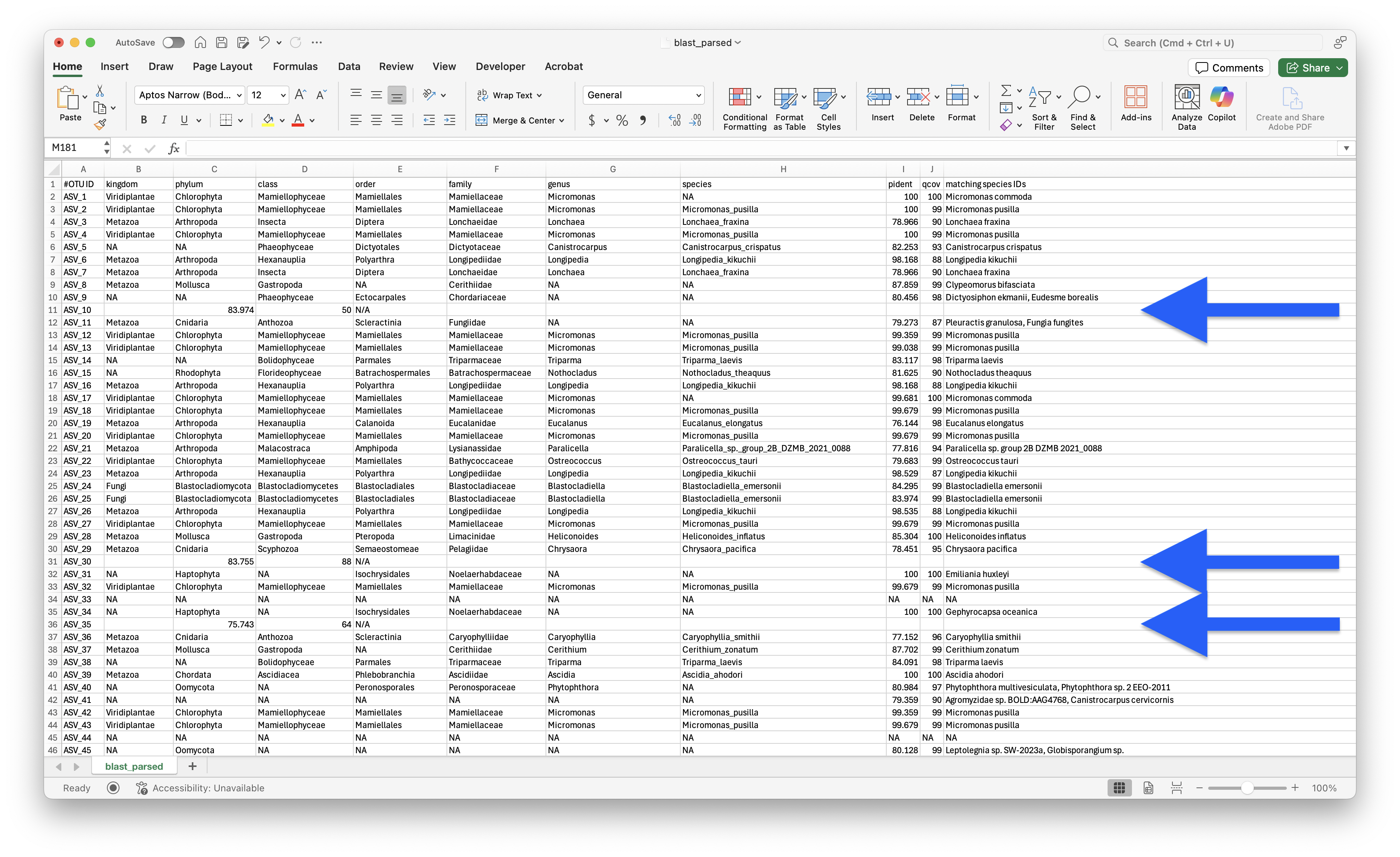
Fig. 39 : A screenshot of the parsing error in the ALEX output file#
When encountering such an issue, standard functions likely are not applicable and custom functions might need to be written.
Luckily, in this case, the custom function is quite “simple”. Namely, we will read the file line by line, rather than as an R dataframe. We then loop over the line and count the number of columns in the line. If the line has the correct number of columns (11 in our case), we can keep the line as is, otherwise, we will rework the line by adding NA in between the ASV name and the BLAST values. Next, we transform the lines as a dataframe and set the first column as row names and first row as column names.
## set function to read in the taxonomy file due to formatting error in ALEX
process_line <- function(line) {
  elements <- unlist(strsplit(line, "\t"))
  if (length(elements) == 11) {
    return(elements)
  }
  if (length(elements) != 11) {
    return(c(elements[1], rep(NA, 7), elements[3:5]))
  }
}

# read and format taxonomy file with ASV IDs as row names and metadata as column names
lines <- readLines(file.path("4.results", "blast_parsed.txt"))
processed_data <- lapply(lines, process_line)
taxonomy <- as.data.frame(do.call(rbind, processed_data), stringsAsFactors = FALSE)
colnames(taxonomy) <- taxonomy[1,]
taxonomy <- taxonomy[-1,]
rownames(taxonomy) <- taxonomy[,1]
taxonomy <- taxonomy[,-1]
3.2 Updating files#
Linked dataframes
It is important to note that the 4 files we just read into R should be seen as “linked together”, meaning that if we were to change one file, we need to keep in mind to alter the other documents as well. The reason for this is that sample and sequence names need to be matching between the documents. Otherwise errors will occur. So, for example, if we remove a sequence from the count table, as it is deemed a contaminant, we need to remove the sequence in the ASV sequence file and taxonomic ID from the taxonomy table as well to keep the sequence lists between these 3 files identical (the fourth file, the metadata file, does not contain information on sequences, so won’t need to be updated in this case).
On the note of the warning, we can see that most dimensions between the 4 dataframes are identical. The count_table has 2,729 obs. (rows as ASV IDs) and 45 variables (columns as sample IDs). sequences is a list of 2,729 elements, identical to the row count of count_table. metadata, on the other hand, has 45 obs. (rows as sample IDs), identical to the column count of count_table. taxonomy, however, has 8,315 obs (rows as ASV IDs)! Remember that this is the original number of ASVs we observed and we still need to remove the rows that were deemed artefacts by tombRaider. So, let’s do that now.
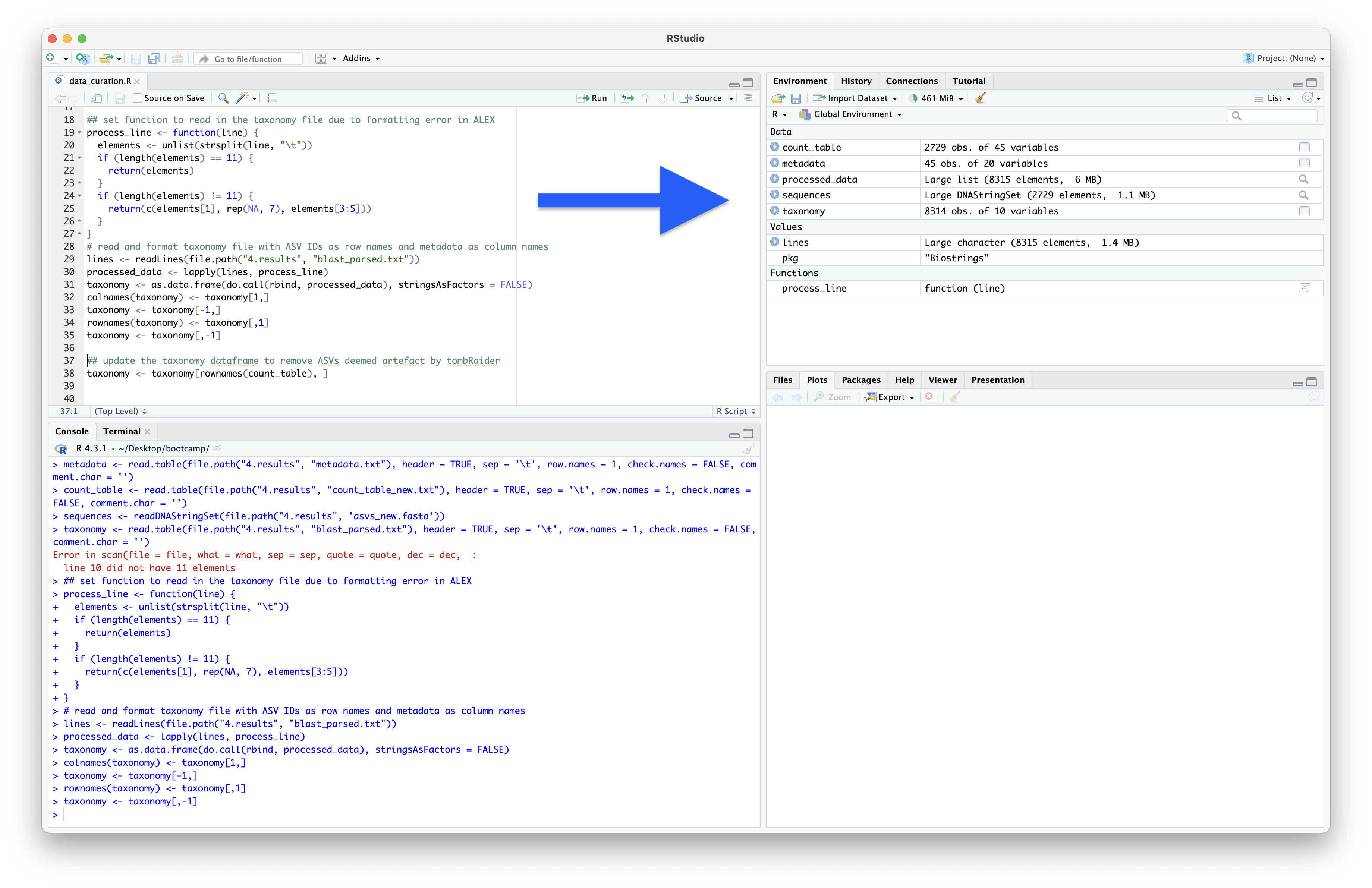
Fig. 40 : Linking files before updating taxonomy#
## update the taxonomy dataframe to remove ASVs deemed artefact by tombRaider
taxonomy <- taxonomy[rownames(count_table), ]
After updating taxonomy, you should now see that the dataframe only consists of 2,729 obs., identical to count_table.
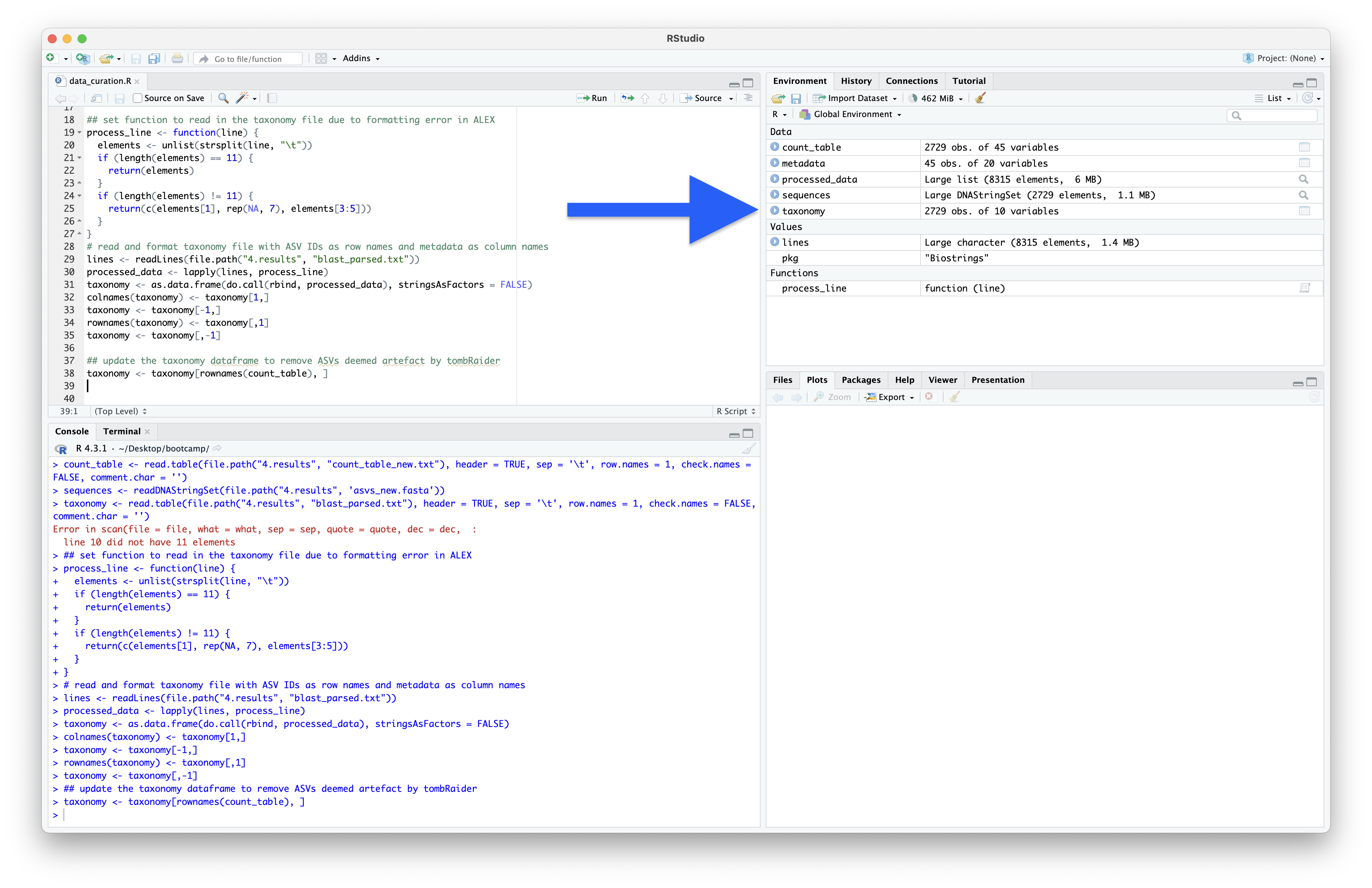
Fig. 41 : Linking files after updating taxonomy#
3.3 Contamination investigation#
Before we remove the contaminant signals from our data, it can be useful to print them out, to determine the seriousness of the contamination in your data. For our tutorial dataset, we have 6 negative control samples, including 3 Field controls (FieldControl_112122, FieldControl_112222, and FieldControl_112422) and 3 Filter controls (FilterControl_112122, FilterControl_112222, and FilterControl_112422). It is possible to link negative control samples to specific samples in your dataset, based on when samples and negative controls were collected, and process them separately. However, in our workshop, we will take a global approach to keep things simple and treat the 6 negative controls as controls for all eDNA samples.
To investigate contaminant signals, it is easier to create a new dataframe that contains all the potential information we might need, including:
Only ASVs that have a positive signal in the negative control samples to keep the new dataframe small;
A column with the total read count across all 6 negative control samples;
A column with the number of times the ASV had a positive detection in the control sample;
A column containing the species ID from the taxonomy assignment;
A column containing the actual ASV sequence, in case we want to investigate further and BLAST the sequence manually.
## create negative control dataframe
negative_controls <- count_table %>%
  select(contains("Control")) %>%
  transmute(read_count = rowSums(.), detections = rowSums(. > 0)) %>%
  filter(read_count != 0 & detections != 0) %>%
  mutate(matching_species_IDs = taxonomy[rownames(.), "matching species IDs"],
         sequence = as.character(sequences[rownames(.)]))
Once we have this new dataframe created, we can use the summarize() function in the tidyverse R package to gather some details.
## explore negative_controls
negative_controls %>%
  summarize(
    neg_asvs = nrow(negative_controls),
    asvs_pct = round(nrow(negative_controls) / nrow(count_table) * 100, 2),
    neg_reads = sum(read_count),
    read_pct = round(sum(read_count) / sum(count_table) * 100, 2),
    single_detections = sum(detections == 1),
    max_detections = sum(detections == 6))
Output
  neg_asvs asvs_pct neg_reads read_pct single_detections max_detections
1       36     1.32     39737      1.1                27              2
Based on the output, we can see that we detected 36 ASVs in negative control samples, accounting for 1.32% of total ASVs. We also observed a total of 39,737 (1.1%) reads across all negative controls. Most detections (27 ASVs), however, were only observed once across all 6 negative control samples, while only 2 ASVs were observed in all 6 negative control samples.
3.4 The Decontam R package#
Once we have explored what is in our negative controls, we are ready to identify actual contaminant signals and remove them based on the Decontam R package.
The first step of the Decontam documentation is to inspect the library sizes for each sample. Luckily, we already have all the necessary information stored in our metadata dataframe, whereby metadata$nonchimera_reads contains the number of reads per sample and metadata$sampleType holds the information if a sample is a negative control or actual eDNA sample.
## inspect library sizes
# calculate medians for each group
medians <- metadata %>%
  group_by(sampleType) %>%
  summarise(median_reads = median(nonchimera_reads))

# plot data
ggplot(data = metadata, aes(x = reorder(rownames(metadata), nonchimera_reads), y = nonchimera_reads, color = sampleType)) +
  geom_point(size = 3, alpha = 0.8) +
  geom_hline(data = medians, aes(yintercept = median_reads, color = sampleType),
             linetype = "dashed", linewidth = 0.7, show.legend = FALSE) +
  geom_text(data = medians, aes(x = nrow(metadata) * 0.9, y = median_reads,
                                label = paste("Median:", comma(median_reads)), color = sampleType),
            hjust = 0, vjust = -0.5, size = 3.5, show.legend = FALSE) +
  scale_y_continuous(labels = comma, expand = expansion(mult = c(0.05, 0.15))) +
  scale_x_discrete(expand = expansion(add = c(0.5, 0.05 * nrow(metadata)))) +
  scale_color_manual(values = c("bottled water" = "#E41A1C", "seawater" = "#377EB8")) +
  labs(title = "Library Size Distribution by Sample Type",
       x = "Samples (ordered by library size)", y = "Total read count", color = "Sample Type") +
  theme_minimal(base_size = 12) +
  theme(axis.text.x = element_text(angle = 90, hjust = 1, vjust = 0.5, size = 8),
    panel.grid.major.x = element_blank(), legend.position = "top",
    plot.title = element_text(hjust = 0.5, face = "bold")) +
  guides(color = guide_legend(override.aes = list(size = 5)))
ggsave(filename = file.path("4.results", "library_read_count.png"), plot = last_plot(), bg = "white", dpi = 300)
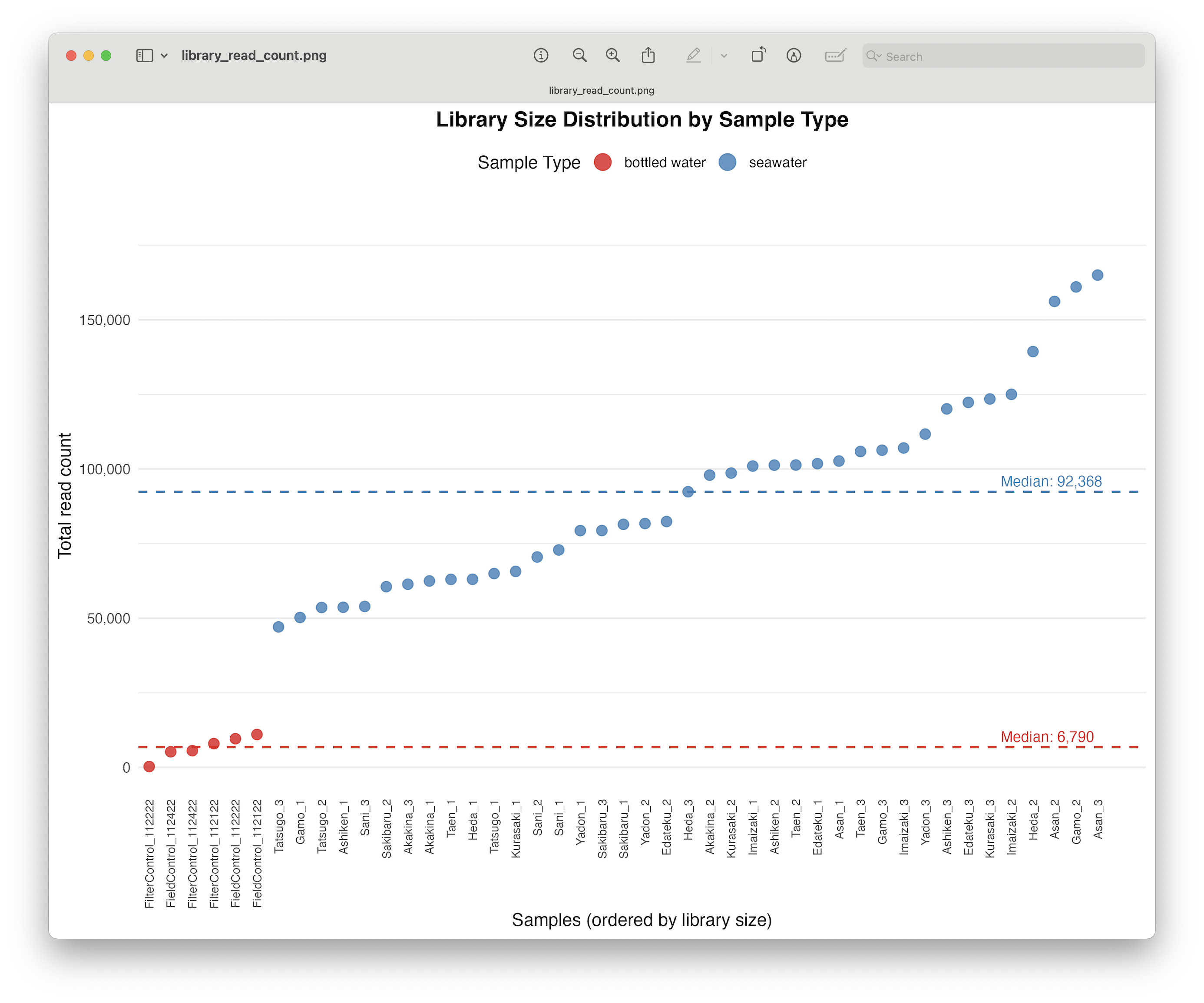
Fig. 42 : Plot depicting read count for each sample in increasing order#
The next step is to create a vector that holds the negative control sample information as a logical variable, with TRUE for negative control samples. It is important that this vector is ordered in the same way as our count table. Rather than manually creating this vector, we can make use of the grepl() function in R.
## determine contaminants using Decontam
# create logical vector
is_control <- grepl("Control", names(count_table), ignore.case = TRUE)
Once we have this vector, we can run the isContaminant() function with method = 'prevalence' to identify contaminants according to the Decontam algorithm. We will set the threshold = 0.51, which will allow Decontam to identify contaminants as all ASVs that are more or equally prevalent in negative control samples than in our eDNA samples. The isContaminant() function will return a dataframe with several columns, with the most important being $p containing the probability for classifying contaminants and $contaminant which contains a logical variable, classifying contaminant ASVs as TRUE based on our threshold value.
# identify contaminants
contaminants <- isContaminant(t(count_table), method = 'prevalence', neg = is_control, threshold = 0.51)
table(contaminants$contaminant)
Output
FALSE  TRUE
 2714    15
Our output shows that Decontam identified 15 ASVs as contaminants, out of the 36 ASVs with a positive identification in negative control samples.
Interestingly, there is currently a bug in the Decontam R package, whereby ASVs present in a single negative control, but absent in all eDNA samples are not identified as contaminants. To fix this issue, let’s build a new dataframe that contains information on (i) the number of detections in negative controls, (ii) the number of detections in our samples, and (iii) the logical variable in column contaminants$contaminant providing the information if Decontam identified an ASV as a contaminant or not. Next, we can set the ASVs with a prevalence of 1 in negative controls and 0 in eDNA samples as TRUE in the contaminant column. Finally, we can print out the results by using the table() function.
# generate summary table and fix bug in Decontam
detection_summary <- count_table %>%
  mutate(detections_in_controls = rowSums(select(., which(is_control)) > 0),
    detections_in_samples = rowSums(select(., which(!is_control)) > 0)) %>%
  select(detections_in_controls, detections_in_samples) %>%
  mutate(contaminant = contaminants[rownames(.), "contaminant"])
detection_summary <- detection_summary %>%
  mutate(contaminant = ifelse(detections_in_controls == 1 & detections_in_samples == 0, TRUE, contaminant))
table(detection_summary$contaminant)
Output
FALSE  TRUE
 2703    26
Once we have fixed the bug in the Decontam output, we can now see that we have identified 26 out of 36 ASVs with a positive identification in negative control samples as contaminant signals. To visualise the process of the Decontam algorithm, we can make use of our newly-created detection_summary dataframe and plot the prevalence of ASV detection between negative controls and eDNA samples.
# plot prevalence and colour by logical contaminant variable
ggplot(data = detection_summary, aes(x = detections_in_controls, y = detections_in_samples, color = contaminant)) +
  geom_abline(intercept = 0, slope = sum(is_control == FALSE) / sum(is_control == TRUE), color = "gray40", linetype = "dashed", linewidth = 0.7) +
  geom_point(size = 3, alpha = 0.7, shape = 16) +
  scale_x_continuous(limits = c(0, 6), breaks = seq(0, 6, by = 1)) +
  scale_y_continuous(limits = c(0, 39), breaks = seq(0, 40, by = 5)) +
  scale_color_manual(values = c("TRUE" = "#E41A1C", "FALSE" = "#377EB8"), name = "Contaminant Status",
                     labels = c("TRUE" = "Contaminant", "FALSE" = "Not Contaminant")) +
  labs(title = "ASV Prevalence in Samples vs Negative Controls", subtitle = "Diagonal line indicates equal prevalence in both groups",
       x = "Prevalence in Negative Controls (n detections)", y = "Prevalence in True Samples (n detections)") +
  theme_minimal(base_size = 12) +
  theme(panel.grid.minor = element_blank(), panel.grid.major = element_line(linewidth = 0.2),
    legend.position = "top", plot.title = element_text(face = "bold", hjust = 0.5), plot.subtitle = element_text(hjust = 0.5, color = "gray40"),
    axis.line = element_line(color = "black"), aspect.ratio = 1) +
  annotate("text", x = 4, y = 28, label = "Equal prevalence line", color = "gray40", size = 3.5, angle = 45)
ggsave(filename = file.path("4.results", "asv_prevalence.png"), plot = last_plot(), bg = "white", dpi = 300)
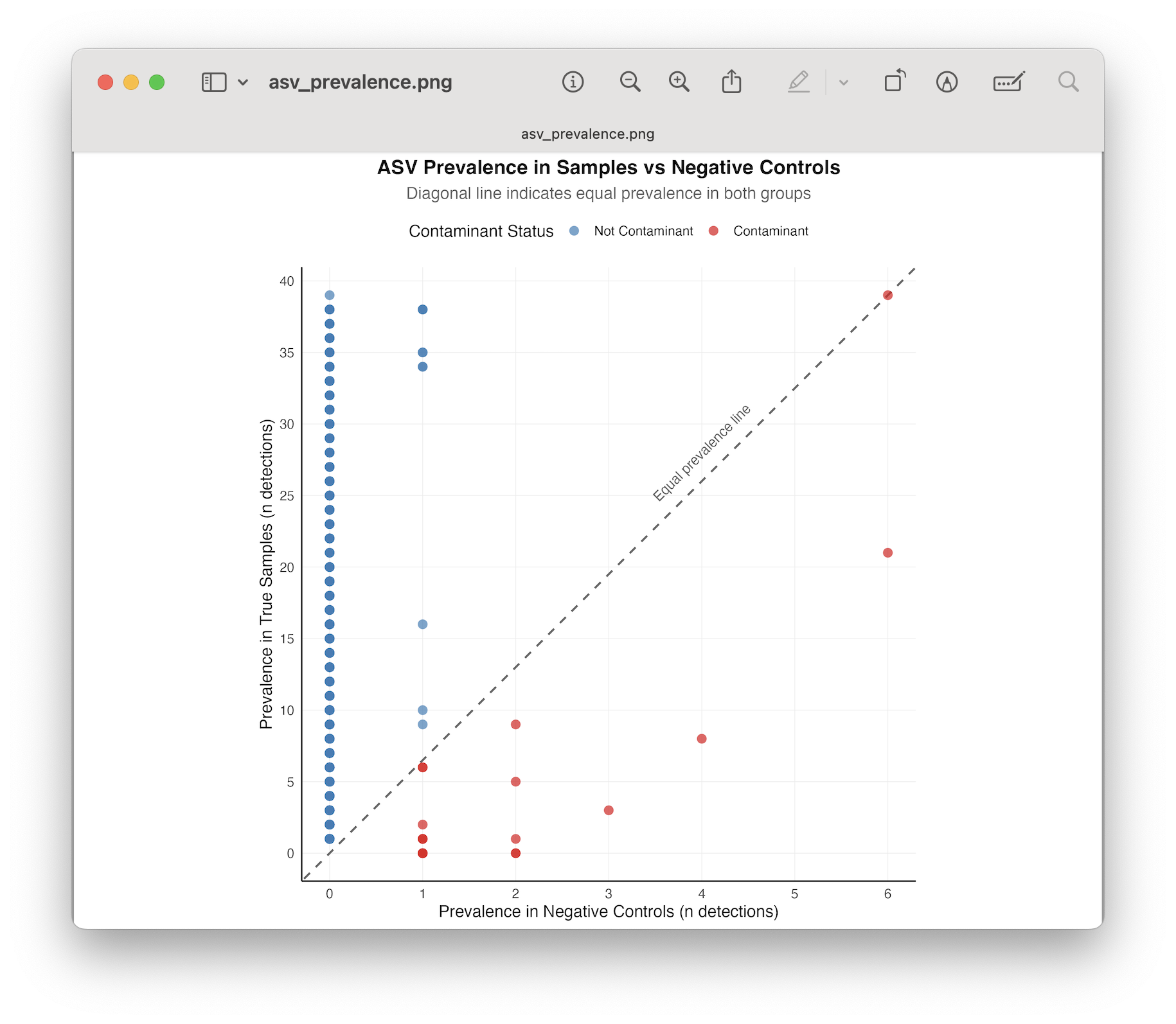
Fig. 43 : The prevalence of detections of sequences in negative controls and true samples#
The final step is to subset the count_table, sequences, and taxonomy dataframes to exclude the contaminant signals from our data and explore the data lost by contamination filtering.
# remove contaminant signals and negative controls from dataframes
contaminant_asvs <- row.names(detection_summary[detection_summary$contaminant == TRUE, ])
count_table_clean <- count_table[!row.names(count_table) %in% contaminant_asvs, ]
count_table_clean <- count_table_clean[, !is_control]
taxonomy_clean <- taxonomy[!row.names(taxonomy) %in% contaminant_asvs, ]
sequences_clean <- sequences[row.names(count_table_clean)]
metadata_clean <- metadata[colnames(count_table_clean), ]

# explore the cleaned count table
sum(count_table) - sum(count_table_clean)
sum(count_table_clean) / sum(count_table) * 100
names(count_table_clean)[colSums(count_table_clean) == 0]
names(count_table_clean)[rowSums(count_table_clean) == 0]
Output
> sum(count_table) - sum(count_table_clean)
[1] 171482
> sum(count_table_clean) / sum(count_table) * 100
[1] 95.27217
> names(count_table_clean)[colSums(count_table_clean) == 0]
character(0)
> names(count_table_clean)[rowSums(count_table_clean) == 0]
character(0)
The Decontam R package identified 26 ASVs as contaminant signals. After removing them from count_table, as well as the negative control samples, we lost 171,482 (4.7%) reads. No sample drop out was observed during contaminant filtering, i.e., no samples obtained 0 reads after removing contaminant signals.
4. Amplicon length filtering#
For amplicons with highly-conserved fragment sizes, such as the 313 bp fragment of the COI amplicon we are analysing in this dataset, we can plot the distribution of amplicons lengths and, potentially, filter out any signals that are outside the range of the expected fragment size. Please note that this is only possible for primer sets that amplify a consistent fragment size across their target taxonomic groups. For some metabarcoding primer sets, this might not be the case. If you are unsure about the amplicon size range for your primer set, you can investigate the amplicon length of the barcodes in your custom reference database using CRABS’ --amplicon-length-figure function, which provides a line graph of the amplicon sizes per taxonomic group.
To visualise the amplicon size distribution of our ASVs, we can extract the sequence length from the sequences object and add the length information to our taxonomy dataframe.
## amplicon length filtering
# extract amplicon lengths and add to taxonomy
taxonomy_clean$sequence_length <- setNames(width(sequences_clean), names(sequences_clean))[rownames(taxonomy_clean)]
Next, we can plot the amplicon size distribution using the geom_density() function in ggplot2, as well as print the values of the number of ASVs shorter than 311 bp or longer than 315 bp.
# plot the amplicon length distribution using a density plot
ggplot(taxonomy_clean, aes(x = sequence_length)) +
  geom_density(fill = "#377EB8", alpha = 0.3, color = "#377EB8", linewidth = 0.5) +
  geom_vline(aes(xintercept = mean(sequence_length)), color = "gray40", linetype = "dashed", linewidth = 0.5) +
  geom_vline(aes(xintercept = min(sequence_length)), color = "gray40", linetype = "dashed", linewidth = 0.5) +
  geom_vline(aes(xintercept = max(sequence_length)), color = "gray40", linetype = "dashed", linewidth = 0.5) +
  theme_minimal(base_size = 12) +
  theme(panel.grid.minor = element_blank(), panel.grid.major = element_line(linewidth = 0.2, color = "gray90"),
    plot.title = element_text(hjust = 0.5, face = "bold"), axis.line = element_line(color = "black")) +
  labs(title = "Distribution of Amplicon Sequence Lengths", x = "Sequence Length (bp)", y = "Density") +
  annotate("text", x = mean(taxonomy_clean$sequence_length), y = Inf, vjust = 1.5, hjust = -0.1,
           label = paste("Mean:", round(mean(taxonomy_clean$sequence_length)), "bp"), color = "gray40") +
  annotate("text", x = min(taxonomy_clean$sequence_length), y = Inf, vjust = 1.5, hjust = -0.1,
           label = paste("Min:", min(taxonomy_clean$sequence_length), "bp"), color = "gray40") +
  annotate("text", x = max(taxonomy_clean$sequence_length), y = Inf, vjust = 1.5, hjust = 1.1,
           label = paste("Max:", max(taxonomy_clean$sequence_length), "bp"), color = "gray40") +
  scale_x_continuous(breaks = pretty_breaks(n = 10)) +
  scale_y_continuous(expand = expansion(mult = c(0, 0.1)))
ggsave(filename = file.path("4.results", "amplicon_length_distribution.png"), plot = last_plot(), bg = "white", dpi = 300)
sum(taxonomy_clean$sequence_length < 311)
sum(taxonomy_clean$sequence_length > 315)
Output
> sum(taxonomy_clean$sequence_length < 311)
[1] 62
> sum(taxonomy_clean$sequence_length > 315)
[1] 50
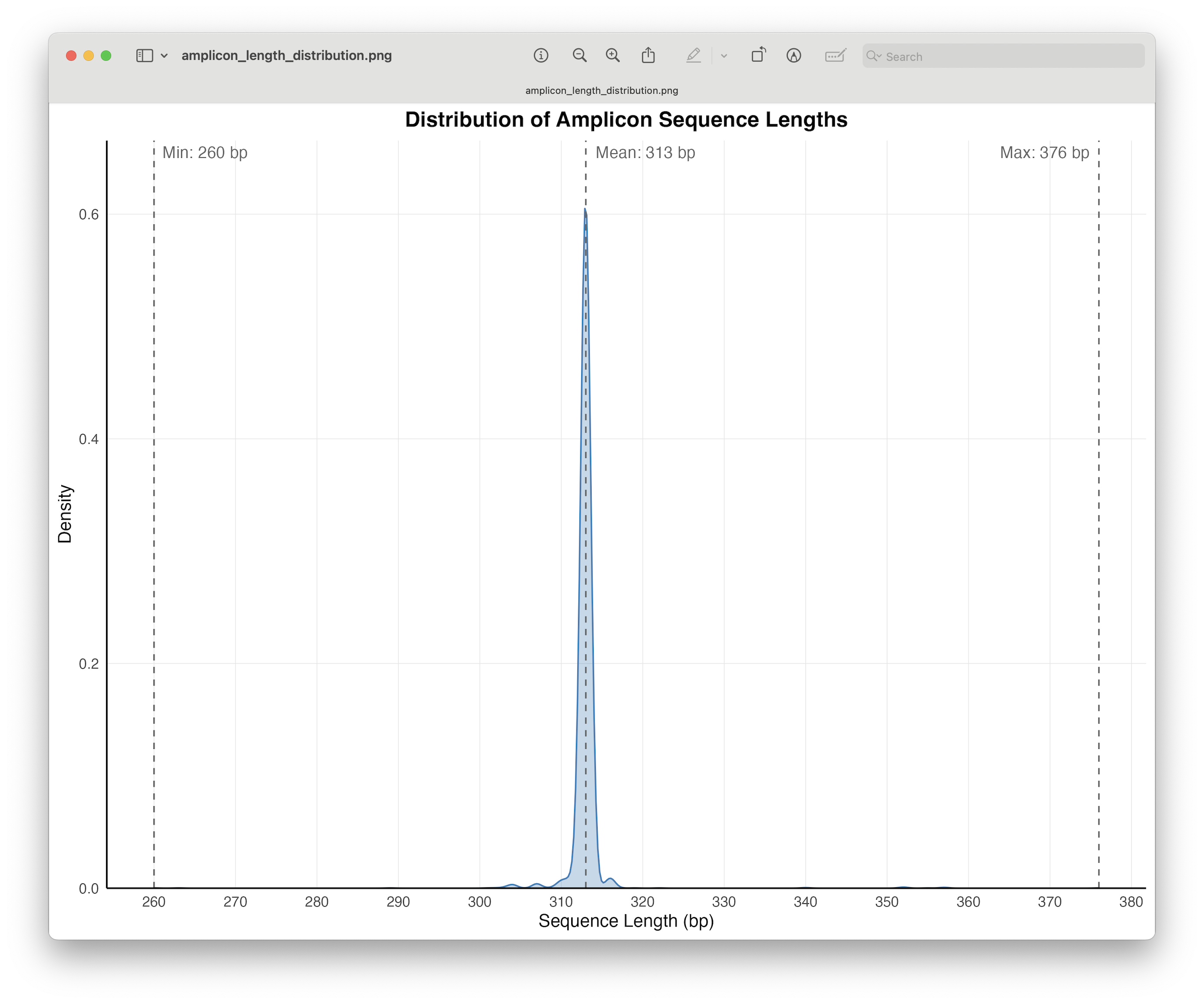
Fig. 44 : A density graph depicting the amplicon length distribution of our COI ASVs#
The output and graph show us that most amplicons are indeed of length 313 bp. However, we have 62 amplicons shorter than 311 bp, with the shortest amplicon length observed as 260 bp, and 50 amplicons longer than 315 bp, with the longest amplicon length observed as 376 bp. Let’s remove those short and long ASVs and update our files again before continuing with the next step.
# remove short and long ASVs, as well as update all dataframes
taxonomy_length <- taxonomy_clean %>%
  filter(sequence_length >= 311, sequence_length <= 315)
count_table_length <- count_table_clean[row.names(taxonomy_length), ]
names(count_table_length)[colSums(count_table_length) == 0]
names(count_table_length)[rowSums(count_table_length) == 0]
sequences_length <- sequences_clean[row.names(count_table_length)]
metadata_length <- metadata_clean
sum(count_table_clean) - sum(count_table_length)
sum(count_table_length) / sum(count_table_clean) * 100
Output
> sum(count_table_clean) - sum(count_table_length)
[1] 87644
> sum(count_table_length) / sum(count_table_clean) * 100
[1] 97.46371
Filtering the data based on amplicon length removed an additional 87,644 (2.5%) reads from the data, though no samples dropped out after this filtering step.
5. Abundance filtering#
5.1 Low abundant detections#
One frequently-included processing step for metabarcoding data is to remove low abundant detections, i.e., detections that are made up by a single or a few reads. This pre-processing step is conducted to minimise the risk of cross-contamination between samples or to elimitate the effect of tag jumps. Tag jumps are sequences that have been assigned to the wrong sample, i.e., contain the wrong tags or barcodes. For more information, I suggest reading this excellent paper by Schnell et al., 2015. Currently, there is no consensus within the metabarcoding research community on the thresholds for abundance filtering and, therefore, is mainly user-defined. Ideally, positive controls are included in the experiment, which can provide insights into the threshold at which background noise enters the dataset. Alternative approaches are to remove singleton detections or detections based on the total read abundance for each ASV independently. Before filtering low-abundant detections, let’s first plot the distribution of detections to investigate the detections present in our dataset.
## abundance filtering
# pivot data to long format and count frequencies
detection_abundance <- count_table_length %>%
  pivot_longer(everything()) %>%
  filter(value > 0) %>%
  count(value) %>%
  uncount(weights = n)

# plot using geom_density
ggplot(detection_abundance, aes(x = value)) +
  geom_density(fill = "#377EB8", alpha = 0.3, color = "#377EB8", linewidth = 0.5, adjust = 1) +
  theme_minimal(base_size = 12) +
  theme(panel.grid.minor = element_blank(), panel.grid.major = element_line(linewidth = 0.2, color = "gray90"),
    plot.title = element_text(hjust = 0.5, face = "bold"), axis.line = element_line(color = "black")) +
  labs(title = "Density Distribution of Non-Zero Values", x = "Value", y = "Density") +
  scale_y_continuous(expand = expansion(mult = c(0, 0.1))) +
  scale_x_log10(labels = trans_format("log10", math_format(10^.x)))
ggsave(filename = file.path("4.results", "detection_frequencies.png"), plot = last_plot(), bg = "white", dpi = 300)
sum(count_table_length == 1)
sum(count_table_length == 2)
Output
> sum(count_table_length == 1)
[1] 11
> sum(count_table_length == 2)
[1] 1078
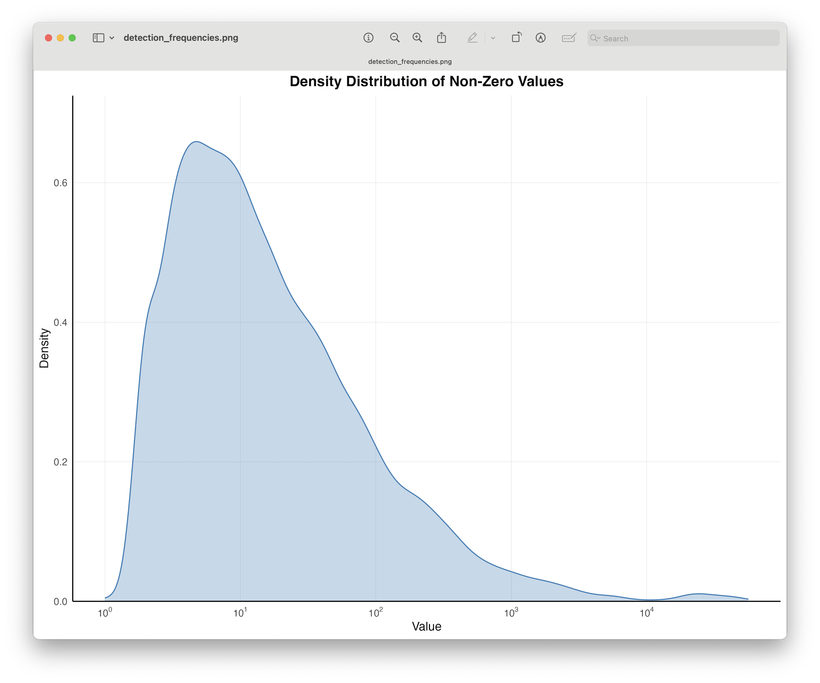
Fig. 45 : A density graph depicting frequency of detections based on read count#
The output shows us that the number of singleton detections in our data is quite low and only appears 11 times in our dataset. The highest number of times a detection was recorded was a read count of 3 with 1,158 detections, followed by a read count of 2 with 1,078 detections, and a read count of 4 with 1,034 detections.
For this workshop, we will remove singleton detections from the dataset.
# remove singleton detections
count_table_length[count_table_length < 2] <- 0
min(count_table_length[count_table_length != 0], na.rm = TRUE)
names(count_table_length)[colSums(count_table_length) == 0]
names(count_table_length)[rowSums(count_table_length) == 0]
Output
> min(count_table_length[count_table_length != 0], na.rm = TRUE)
[1] 2
> names(count_table_length)[colSums(count_table_length) == 0]
character(0)
> names(count_table_length)[rowSums(count_table_length) == 0]
character(0)
5.2 Low abundant ASVs#
Besides low abundant detections, low abundant ASVs are also frequently removed from the data. For pipelines employing USEARCH/VSEARCH during denoising, ASVS with an abundance less than 8 are by default removed by the algorithm. Other applications, such as SWARM and dada2 do not have this abundance threshold built in by default. Hence, let’s investigate the abundance distribution of ASVs in our data.
# reformat data to fit geom_density
asv_abundance <- count_table_length %>%
  mutate(value = rowSums(.)) %>%
  select(value)

# plot using geom_density
ggplot(asv_abundance, aes(x = value)) +
  geom_density(fill = "#377EB8", alpha = 0.3, color = "#377EB8", linewidth = 0.5, adjust = 1) +
  geom_vline(aes(xintercept = 8), color = "gray40", linetype = "dashed", linewidth = 0.5) +
  theme_minimal(base_size = 12) +
  theme(panel.grid.minor = element_blank(), panel.grid.major = element_line(linewidth = 0.2, color = "gray90"),
        plot.title = element_text(hjust = 0.5, face = "bold"), axis.line = element_line(color = "black")) +
  labs(title = "Density Distribution of Non-Zero Values", x = "Value", y = "Density") +
  scale_y_continuous(expand = expansion(mult = c(0, 0.1))) +
  scale_x_log10(labels = trans_format("log10", math_format(10^.x))) +
  annotate("text", x = 8, y = Inf, vjust = 1.5, hjust = -0.1,
           label = paste("Traditional ASV cutoff\nat read abundance = 8"), color = "gray40")
sum(asv_abundance < 8)
round(sum(asv_abundance < 8)  / nrow(asv_abundance) * 100, 2)
Output
> sum(asv_abundance < 8)
[1] 859
> round(sum(asv_abundance < 8)  / nrow(asv_abundance) * 100, 2)
[1] 33.15
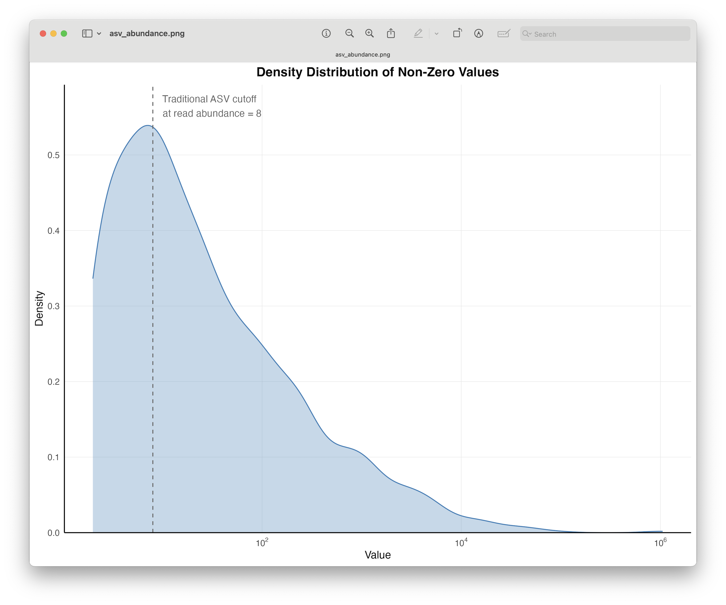
Fig. 46 : A density graph depicting ASV abundance in our COI dataset#
The output shows that 859 ASVs or 33.15% have an abundance lower than 8 reads. As it is a standard approach to remove these low-abundant signals, let’s do this as well for our tutorial data. Note that for your own data, you might want to explore the taxonomic ID of these signals more in depth before deciding to remove them.
# remove low abundant asvs, update the tables, and explore lost reads
count_table_high <- count_table_length[rowSums(count_table_length) > 7, ]
names(count_table_length)[colSums(count_table_length) == 0]
names(count_table_length)[rowSums(count_table_length) == 0]
metadata_high <- metadata_length
sequences_high <- sequences_length[row.names(count_table_high)]
taxonomy_high <- taxonomy_length[row.names(count_table_high), ]
sum(count_table_length) - sum(count_table_high)
sum(count_table_high) / sum(count_table_length) * 100
Output
> sum(count_table_length) - sum(count_table_high)
[1] 3398
> sum(count_table_high) / sum(count_table_length) * 100
[1] 99.89911
Removing the 859 low-abundant ASVs, only resulted in the loss of 3,398 (0.1%) reads, while no samples dropped out during this filtering step.
6. Rarefaction#
The second-to-last data curation step we will introduce during this workshop is how to deal with differences in sequencing depth between samples and assess if sufficient sequencing depth was achieved for each sample. With the realisation that a higher read count could lead to a larger number of ASVs being detected, there has been much debate in the scientific community on how to deal with this issue. Some studies argue that it is essential to “level the playing field” and use the same number of sequences across all samples. This random subsampling of the data is called rarefaction. See Cameron et al., 2021 as an example. Other studies, on the other hand, argue vehemently agains such an approach. For example, you can read McMurdie et al., 2014 for more on this topic. While this debate is still ongoing, I suggest to run a couple of statistical tests and visualisations that can help determine the need to rarefy your data. Afterwards, you can make an informed decision and clearly state why or why not you have decided to process your data in a certain way.
I suggest to run 4 tests to determine if rarefying your data might be necessary, including:
determine if there is a big difference in read count between samples;
determine if there is a positive correlation between sequencing depth and number of observed ASVs;
draw so-called rarefaction curves to determine if sufficient sequencing coverage has been achieved; and
calculate curvature indices to provide a statistical test regarding the observed patterns in rarefaction curves.
6.1 Read distribution#
As a first test, we can plot the read distribution for samples as a visualisation. For easy viewing, we can colour the bars and boxes based on the metadata file. As a statistical test, we can run a one-way ANOVA to determine significant differences in read count between sample locations. However, with a replication of n = 3, even the non-parametric alternative might not be highly accurate.
## rarefaction
# read distribution
# add column sums of count_table_high to metadata_table_high
metadata_high$total_read_count <- colSums(count_table_high)[rownames(metadata_high)]

# plot total read count in decreasing order with transformed and untransformed y-axes
sample_colors <- c("Akakina" = "#EAE0DA", "Asan" = "#A0C3D2", "Ashiken" = "#E7C8C0", "Edateku" = "#B5C7A4",
  "Gamo" = "#D4BBDD", "Heda" = "#F2D7A7", "Imaizaki" = "#A2D9D1", "Kurasaki" = "#DFA7A7", "Sakibaru" = "#C5D0E6",
  "Sani" = "#D9C5A0", "Taen" = "#B7D9C4", "Tatsugo" = "#E3B7D1", "Yadon" = "#A8C6D9")
plot_log <- ggplot(metadata_high, aes(x = reorder(row.names(metadata_high), -total_read_count), y = total_read_count, fill = sampleLocation)) +
  geom_col(width = 0.8) +
  scale_fill_manual(values = sample_colors, name = "Sample Location") +
  scale_y_log10(breaks = trans_breaks("log10", function(x) 10^x), labels = trans_format("log10", math_format(10^.x)), expand = expansion(mult = c(0, 0.1))) +
  labs(y = "Total Reads (log10)", x = NULL) +
  theme_minimal(base_size = 12) +
  theme(panel.grid.major.x = element_blank(), panel.grid.minor = element_blank(), axis.text.x = element_blank(), axis.line = element_line(color = "black"), legend.position = "none")
plot_raw <- ggplot(metadata_high, aes(x = reorder(row.names(metadata_high), -total_read_count), y = total_read_count, fill = sampleLocation)) +
  geom_col(width = 0.8) +
  scale_fill_manual(values = sample_colors, guide = "none") +
  scale_y_continuous(labels = comma, expand = expansion(mult = c(0, 0.1))) +
  labs(x = "Sample Location", y = "Total Reads") +
  theme_minimal(base_size = 12) +
  theme(panel.grid.major.x = element_blank(), panel.grid.minor = element_blank(), axis.text.x = element_text(angle = 90, hjust = 1, vjust = 0.5), axis.line = element_line(color = "black"))
combined_plot <- (plot_log / plot_raw) + plot_layout(guides = "collect") +
  plot_annotation(title = "Sample Sequencing Depth", theme = theme(plot.title = element_text(hjust = 0.5, face = "bold"))) +
  theme(legend.position = "bottom", legend.box.margin = margin(t = 10))
ggsave(filename = file.path("4.results", "read_distribution.png"), plot = combined_plot, bg = "white", dpi = 300)
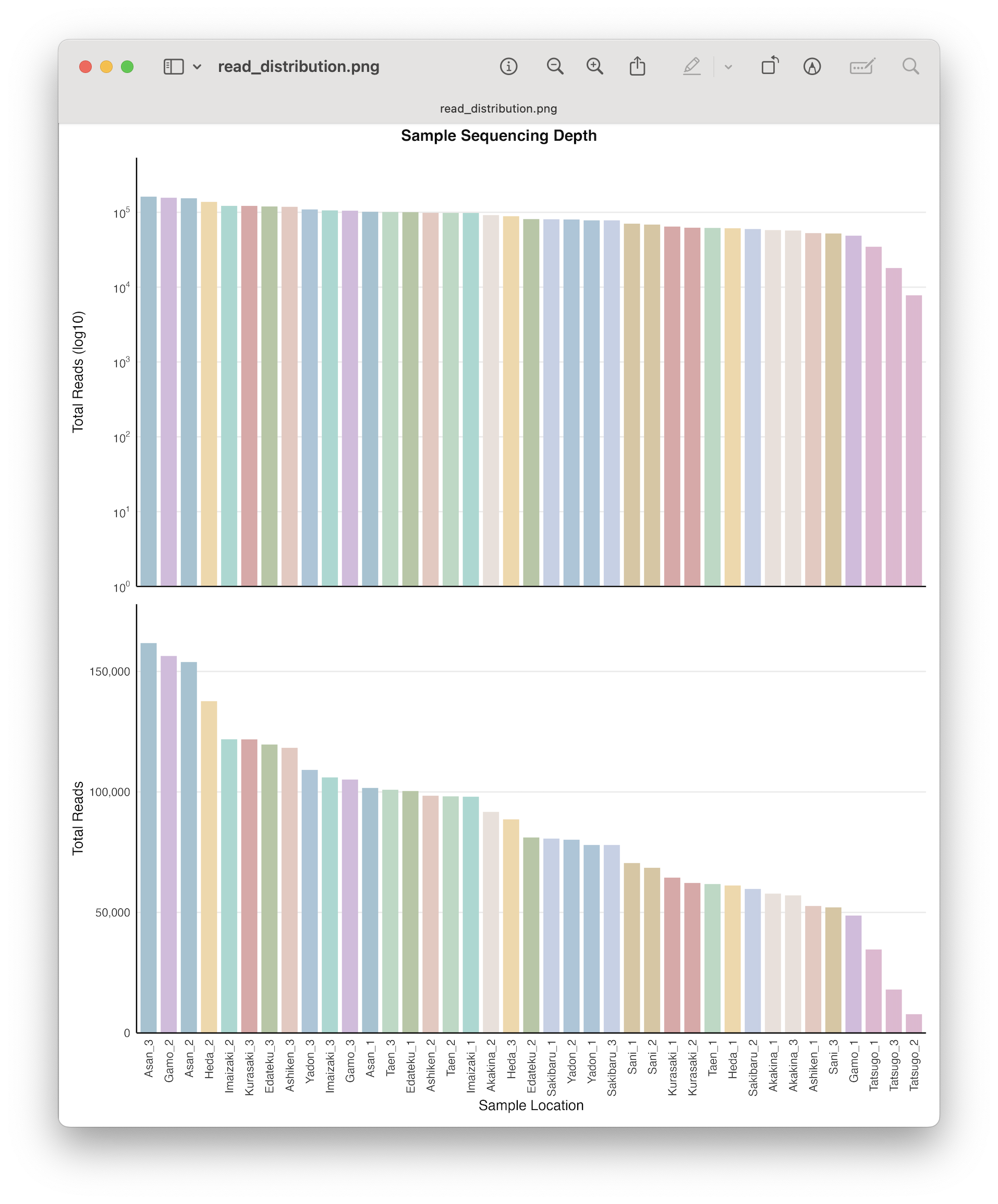
Fig. 47 : The read distribution for samples with and without y-axis log transformation#
Besides a bar graph, a boxplot might be easier to visualise differences between sample locations in read count.
# plot boxplots of read count per group
ggplot(metadata_high, aes(x = sampleLocation, y = total_read_count, fill = sampleLocation)) +
  geom_boxplot() +
  labs(x = "Location", y = "Total Read Count") +
  theme_classic() +
  scale_fill_manual(values = sample_colors) +
  scale_y_continuous(labels = comma, expand = expansion(mult = c(0, 0.1))) +
  labs(x = "Sample Location", y = "Total Reads") +
  theme_minimal(base_size = 12) +
  theme(panel.grid.major.x = element_blank(), panel.grid.minor = element_blank(),
        axis.text.x = element_text(angle = 90, hjust = 1, vjust = 0.5),
        axis.line = element_line(color = "black"), legend.position = "none")
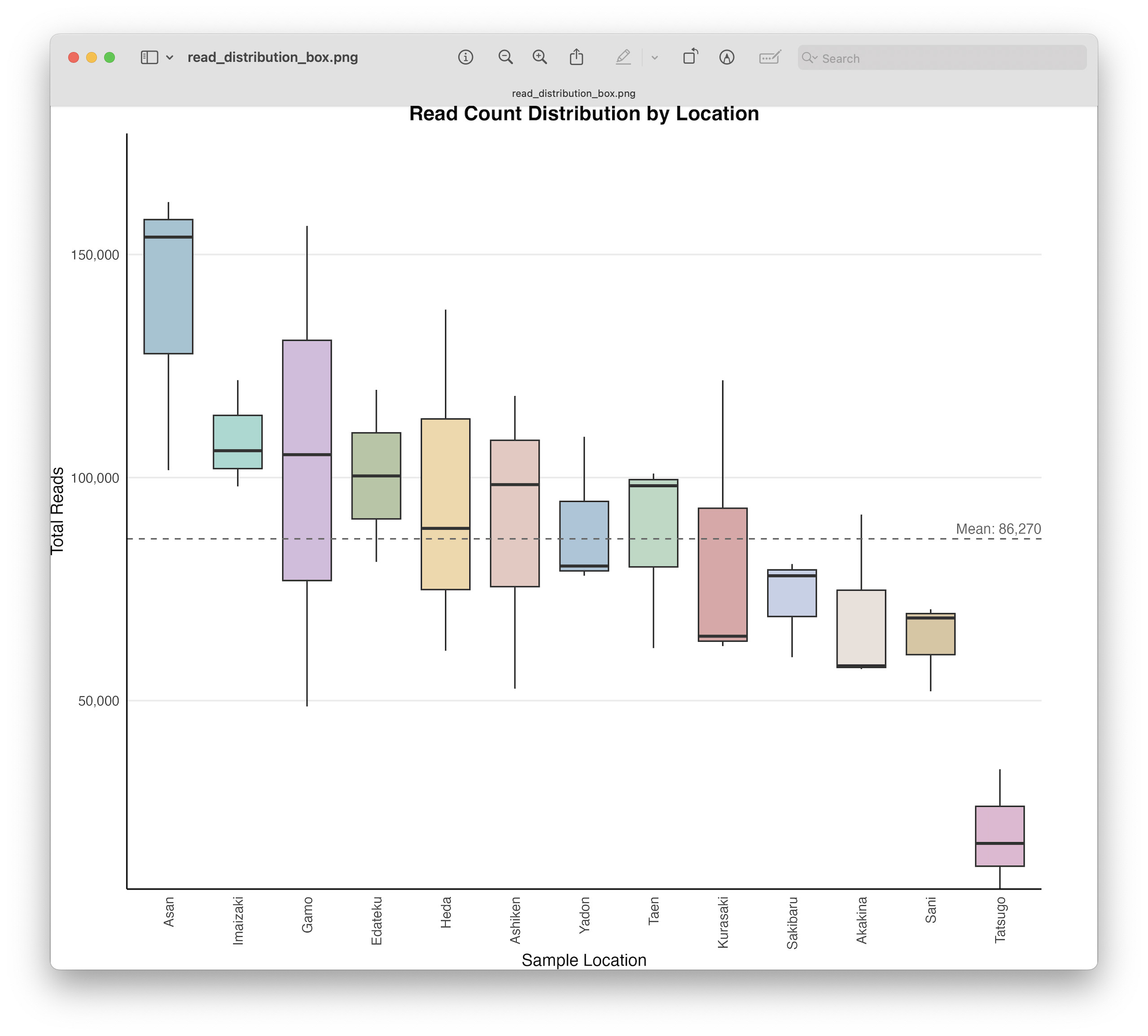
Fig. 48 : The read distribution for samples via a boxplot visualisation#
Based on this figure, we can clearly see that samples from Tatsugo have fewer reads compared to the average, while samples from Asan and Imaizaki have a higher than average read count. Besides a figure, we can also print out the basic information on read count to get an even clearer view.
## print basic stats of read distribution across samples
cat("Maximum value:", max(metadata_high$total_read_count, na.rm = TRUE), "in sample:", rownames(metadata_high)[which.max(metadata_high$total_read_count)], "\n")
cat("Minimum value:", min(metadata_high$total_read_count, na.rm = TRUE), "in sample:", rownames(metadata_high)[which.min(metadata_high$total_read_count)], "\n")
cat("Mean value:", mean(metadata_high$total_read_count, na.rm = TRUE), "\n")
cat("Standard error:", sd(metadata_high$total_read_count, na.rm = TRUE) / sqrt(sum(!is.na(metadata_high$total_read_count))), "\n")

## print basic stats of read distribution between groups
metadata_high %>%
  group_by(sampleLocation) %>%
  summarise(mean_count = mean(total_read_count, na.rm = TRUE), se_count = sd(total_read_count, na.rm = TRUE) / sqrt(n()))
Output
   sampleLocation mean_count se_count
   <chr>               <dbl>    <dbl>
 1 Akakina            68865.   11426.
 2 Asan              139100.   18860.
 3 Ashiken            89801.   19428.
 4 Edateku           100381    11133.
 5 Gamo              103413    31101.
 6 Heda               95818    22368.
 7 Imaizaki          108629.    7003.
 8 Kurasaki           82827    19500.
 9 Sakibaru           72788     6569.
10 Sani               63703     5831.
11 Taen               86951    12609.
12 Tatsugo            20137.    7826.
13 Yadon              89102.   10039.
Finally, we can test if there is a significant difference in read count between locations. As mentioned before, ideally, the level of replication would be higher than 3, especially for statistical analyses. However, collecting 3 replicates is a standard approach for eDNA metabarcoding surveys.
# run one-way ANOVA
metadata_high$total_read_count[is.na(metadata_high$total_read_count)] <- 0
bartlett.test(total_read_count ~ sampleLocation, data = metadata_high)
leveneTest(total_read_count ~ sampleLocation, data = metadata_high)
histogram(~ total_read_count | sampleLocation, data = metadata_high, layout = c(5,3))
model <- lm(total_read_count ~ sampleLocation, data = metadata_high)
Anova(model, type="II")
Anova(model, Type="II", white.adjust=TRUE)
summary(model)
(HSD.test(model, "sampleLocation"))
Output
Bartlett test of homogeneity of variances

data:  total_read_count by sampleLocation
Bartlett's K-squared = 10.851, df = 12, p-value = 0.5418

Levene's Test for Homogeneity of Variance (center = median)
      Df F value Pr(>F)
group 12  0.5452 0.8645
      26

Anova Table (Type II tests)

Response: total_read_count
                   Sum Sq Df F value  Pr(>F)
sampleLocation 2.7827e+10 12   3.061 0.00821 **
Residuals      1.9696e+10 26
Signif. codes:  0 ‘***’ 0.001 ‘**’ 0.01 ‘*’ 0.05 ‘.’ 0.1 ‘ ’ 1

Analysis of Deviance Table (Type II tests)

Response: total_read_count
               Df      F    Pr(>F)
sampleLocation 12 5.4646 0.0001455 ***
Residuals      26
Signif. codes:  0 ‘***’ 0.001 ‘**’ 0.01 ‘*’ 0.05 ‘.’ 0.1 ‘ ’ 1
Both our graph and the statistical tests show us a significant difference in read count between locations. The Tukey HSD multiple comparison identified Asan, Imaizaki, and Gamo to have a significant higher number of reads compared to Tatsugo.
6.2 Read count and ASV number correlation#
To visualise a potential positive correlation between total read count and ASV sequence richness, we can plot the total read count against the total number of observed ASV sequences within samples. To test the significance, we can run a spearman rank corralation or pearson’s correlation test. However, better yet is to fit a GLM model with a poisson log-link function. The reason for this is that a Poisson distribution is more appropriate for count data, which both of our variables are, while a log link function ensures predictions are non-negative.
# correlation
# add ASV count to metadata_high
metadata_high$total_observations <- colSums(count_table_high > 0)[rownames(metadata_high)]

# fit the GLM model
glm_model <- glm(total_observations ~ total_read_count,
                 family = poisson(link = "log"), data = metadata_high)
summary(glm_model)

# make predictions
metadata_high$predicted <- predict(glm_model, type = "response")

# plot results
metadata_high$sampleLocation <- as.factor(metadata_high$sampleLocation)
p <- ggplot(metadata_high, aes(x = total_read_count, y = total_observations, color = sampleLocation)) +
  geom_point(size = 8, alpha = 0.7) +
  scale_color_manual(values = sample_colors) +
  geom_smooth(aes(y = predicted), method = "glm", method.args = list(family = "poisson"),
              se = TRUE, linetype = 'dotdash', color = "black", linewidth = 0.3) +
  labs(color = "Location", x = "Total read count",
       y = "Number of observed ASVs") +
  theme_bw() +
  theme(legend.position = "bottom")
p
p1 <- ggMarginal(p, type = 'densigram')
p1
ggsave(filename = file.path("4.results", "read_asv_correlation.png"), plot = p1, bg = "white", dpi = 300)
Output
Call:
glm(formula = total_observations ~ total_read_count, family = poisson(link = "log"),
    data = metadata_high)

Coefficients:
                  Estimate Std. Error z value Pr(>|z|)
(Intercept)      5.122e+00  2.527e-02  202.64   <2e-16 ***
total_read_count 7.564e-06  2.479e-07   30.51   <2e-16 ***
---
Signif. codes:  0 ‘***’ 0.001 ‘**’ 0.01 ‘*’ 0.05 ‘.’ 0.1 ‘ ’ 1

(Dispersion parameter for poisson family taken to be 1)

    Null deviance: 2354.7  on 38  degrees of freedom
Residual deviance: 1430.3  on 37  degrees of freedom
AIC: 1727.4

Number of Fisher Scoring iterations: 4
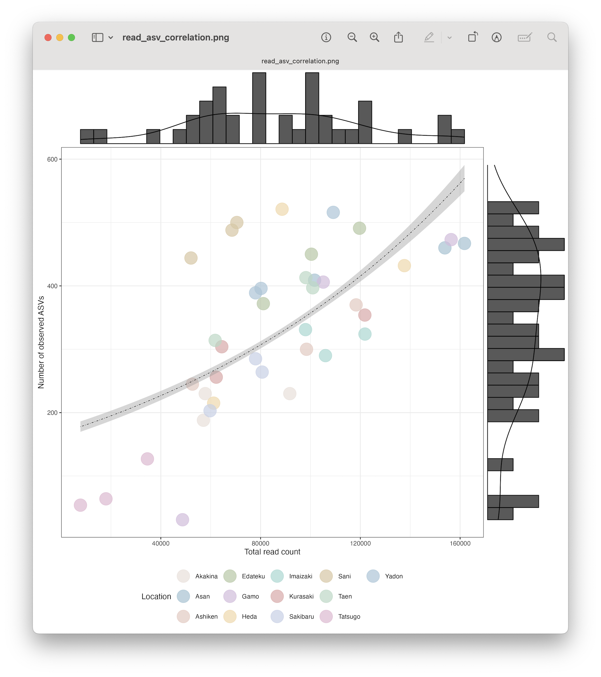
Fig. 49 : The correlation between read count and number of detected ASVs#
From both the GLM and the figure, we can see that there is a significant positive correlation between total read count and number of detected ASVs.
From the plot, we can determine that this significant correlation is likely driven by the low read count samples of Tatsugo, as well as a single outlier sample in Gamo.
From the GLM output, we can determine a highly significant correlation (p < 0.001) between total read count and number of observed ASVs, suggesting a strong positive relationship between the two. More practically, we can infer that for every 1-unit increase in the total read count, the log-count of ASVs increases by 7.564 x 10^-6, or for every 10,000 reads, we expect ASV count to increase by ~1.0785. Furthermore, the large drop between null deviance and residual deviance suggests the predictor (total read count) improves the model. One potential issue with the GLM, however, is that the residual deviance is much larger than the degrees of freedom (1430.3 >> 37). This could mean that the data may be overdispersed and a negative binomial GLM might be more appropriate, as this version accounts for overdispersion, which Poisson regression does not. Another option could be to remove the outliers from the data and see if this fixes the issue.
optimising the GLM
Try re-running the GML with the outliers removed, as well as run a negative binomial GML, to see if this gives us better results.
6.3 Rarefaction curves#
The second-to-last check to see if we might want to rarefy our data, we can draw rarefaction curves and determine if they plateau. These graphs can also be used to determine if sufficient sequencing depth was achieved within our experiment. Such plots, however, need to be conducted on the unfiltered frequency table, as data processing has a major effect on the results of rarefaction curves and skews the data in favour of sufficient sequencing depth. Rarefaction curve plots are frequently included in the supplemental files of metabarcoding publications and referenced to in the manuscript. We can use the amp_rarecurve function in the ampvis2 R package to draw such plots.
# rarefaction plots
# read in the data
count_raw <- read.table(file.path("4.results", "count_table.txt"), header = TRUE, sep = '\t', check.names = FALSE, comment.char = '')
colnames(count_raw)[1] <- "V1"
taxonomy <- as.data.frame(do.call(rbind, processed_data), stringsAsFactors = FALSE)
colnames(taxonomy) <- taxonomy[1,]
taxonomy <- taxonomy[-1,]
colnames(taxonomy)[1] <- "V1"
meta_raw <- read.table(file.path("4.results", "metadata.txt"), header = TRUE, sep = '\t', check.names = FALSE, comment.char = '')

# prepare data for analysis and plotting
count_raw <- merge(count_raw, taxonomy[, c("V1", "matching species IDs")], by = "V1", all.x = TRUE)
colnames(count_raw)[1] <- "ASV"
colnames(count_raw)[ncol(count_raw)] <- "Species"
meta_raw$sampleLocation <- factor(meta_raw$sampleLocation)

# load dataframes into ampvis2 format
ampvis_df <- amp_load(count_raw, meta_raw)

# generate rarefaction curves
rarefaction_curves <- amp_rarecurve(ampvis_df, stepsize = 100, color_by = "sampleLocation") +
  ylab("Number of observed ASVs") +
  theme_classic() +
  scale_color_manual(values = sample_colors) +
  theme(legend.position = "bottom") +
  facet_wrap(~ sampleLocation)
rarefaction_curves
ggsave(filename = file.path("4.results", "rarefaction_curves.png"), plot = rarefaction_curves, bg = "white", dpi = 300)
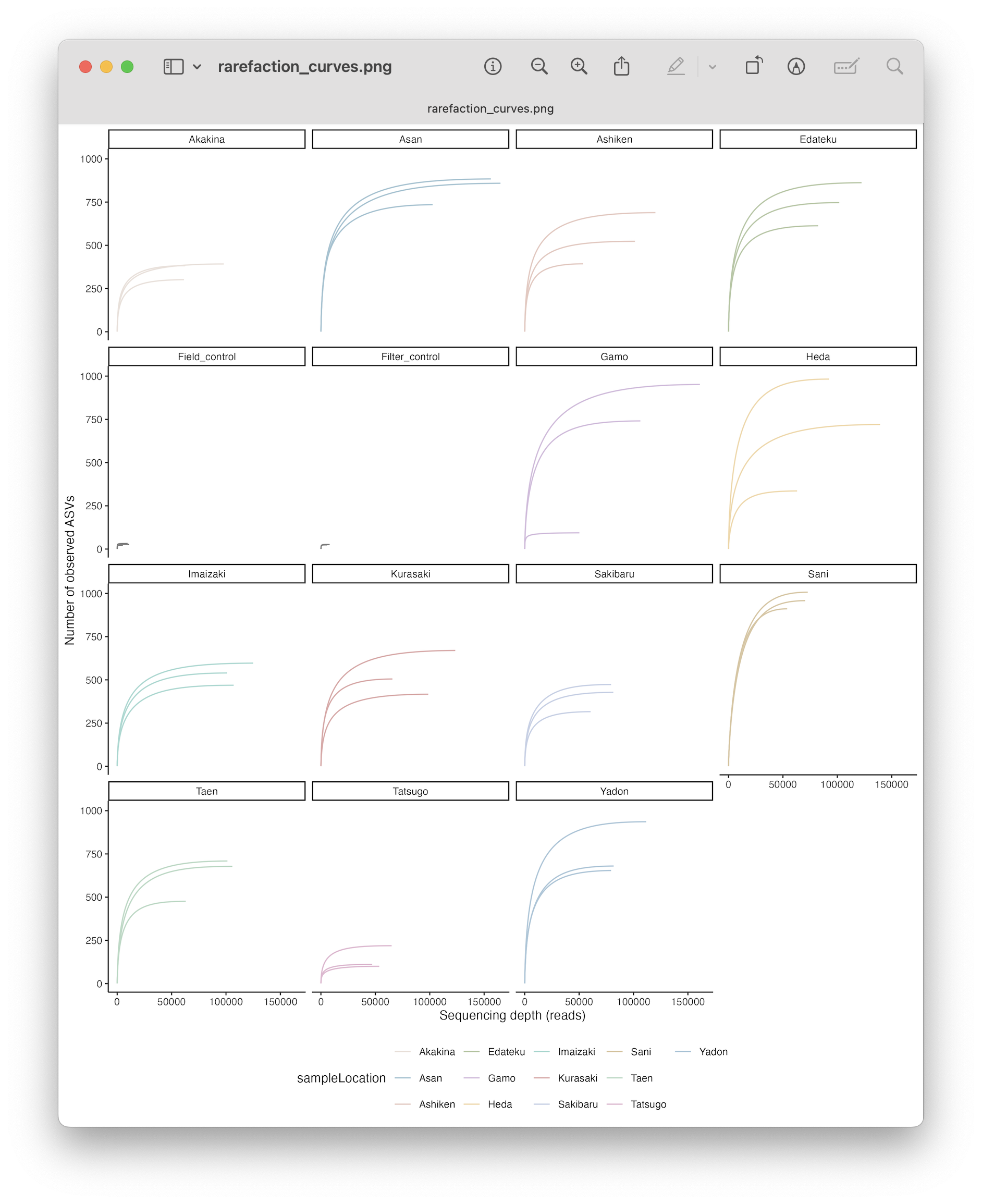
Fig. 50 : Rarefaction curves drawn with the amp_rarecurve() function in the ampvis2 R package.#
From the plot, we can see that most rarefaction curves plateau, indicating sufficient sequencing depth is achieved for this experiment and that additional sequencing might not result in a significantly higher number of ASVs detected.
6.4 Curvature indices#
The final check I recommend running is to help interpret the rarefaction curves. Based on the dimensions of the rarefaction plot used, rarefaction curves might appear as if they flatten while in theory they do not. Calculating curvature indices, i.e., the area under the curve divided by the total plot area, will help mitigate this issue and provide a value for which we can place a threshold to state if a rarefaction curve has flattened or not. We can use the DivSubsamples() and Curvature() functions in the DivE R package to calculate the curvature indices. For more information, I recommend reading the associated paper by Laydon et al., 2014.
# curvature indices
# read in the data
count_raw <- read.table(file.path("4.results", "count_table.txt"), header = TRUE, sep = '\t', check.names = FALSE, comment.char = '')

# create an empty dataframe to place the curvature indices in
curvature_df <- data.frame("sampleID" = numeric(0), "curvature_index" = numeric(0))

# iterate over columns and create new data frames
for (i in 2:ncol(count_raw)) {
  col1_name <- names(count_raw)[1]
  col2_name <- names(count_raw)[i]
  new_df <- data.frame(count_raw[, 1], count_raw[, i])
  names(new_df) <- c(col1_name, col2_name)
  ## function to generate the rarefaction data from a given sample
  dss <- DivSubsamples(new_df, nrf=100, minrarefac=1, NResamples=10)
  ## calculate curvature index
  curvature_value <- Curvature(dss)
  # add info to empty dataframe
  new_row <- data.frame("sampleID" = col2_name, "curvatureIndex" = curvature_value)
  cat("item:", i-1, "/", ncol(count_table), "; sample:", col2_name, "; curvature index: ", curvature_value, "\n")
  curvature_df <- rbind(curvature_df, new_row)
}
Output
item: 1 / 45 ; sample: Akakina_1 ; curvature index:  0.7739905
item: 2 / 45 ; sample: Akakina_2 ; curvature index:  0.8045226
item: 3 / 45 ; sample: Akakina_3 ; curvature index:  0.7803026
item: 4 / 45 ; sample: Asan_1 ; curvature index:  0.7758052
item: 5 / 45 ; sample: Asan_2 ; curvature index:  0.7957316
item: 6 / 45 ; sample: Asan_3 ; curvature index:  0.7954779
item: 7 / 45 ; sample: Ashiken_1 ; curvature index:  0.7771978
item: 8 / 45 ; sample: Ashiken_2 ; curvature index:  0.8133532
item: 9 / 45 ; sample: Ashiken_3 ; curvature index:  0.801376
item: 10 / 45 ; sample: Edateku_1 ; curvature index:  0.7782955
item: 11 / 45 ; sample: Edateku_2 ; curvature index:  0.7839595
item: 12 / 45 ; sample: Edateku_3 ; curvature index:  0.7800647
item: 13 / 45 ; sample: FieldControl_112122 ; curvature index:  0.9119489
item: 14 / 45 ; sample: FieldControl_112222 ; curvature index:  0.9207676
item: 15 / 45 ; sample: FieldControl_112422 ; curvature index:  0.9272206
item: 16 / 45 ; sample: FilterControl_112122 ; curvature index:  0.9110152
item: 17 / 45 ; sample: FilterControl_112222 ; curvature index:  0.7022145
item: 18 / 45 ; sample: FilterControl_112422 ; curvature index:  0.896636
item: 19 / 45 ; sample: Gamo_1 ; curvature index:  0.8864917
item: 20 / 45 ; sample: Gamo_2 ; curvature index:  0.7691496
item: 21 / 45 ; sample: Gamo_3 ; curvature index:  0.7658717
item: 22 / 45 ; sample: Heda_1 ; curvature index:  0.7441417
item: 23 / 45 ; sample: Heda_2 ; curvature index:  0.7689818
item: 24 / 45 ; sample: Heda_3 ; curvature index:  0.7536731
item: 25 / 45 ; sample: Imaizaki_1 ; curvature index:  0.7612742
item: 26 / 45 ; sample: Imaizaki_2 ; curvature index:  0.7839581
item: 27 / 45 ; sample: Imaizaki_3 ; curvature index:  0.7709736
item: 28 / 45 ; sample: Kurasaki_1 ; curvature index:  0.7763308
item: 29 / 45 ; sample: Kurasaki_2 ; curvature index:  0.7649486
item: 30 / 45 ; sample: Kurasaki_3 ; curvature index:  0.7795486
item: 31 / 45 ; sample: Sakibaru_1 ; curvature index:  0.7620652
item: 32 / 45 ; sample: Sakibaru_2 ; curvature index:  0.7625555
item: 33 / 45 ; sample: Sakibaru_3 ; curvature index:  0.7578724
item: 34 / 45 ; sample: Sani_1 ; curvature index:  0.6896348
item: 35 / 45 ; sample: Sani_2 ; curvature index:  0.6820809
item: 36 / 45 ; sample: Sani_3 ; curvature index:  0.6672233
item: 37 / 45 ; sample: Taen_1 ; curvature index:  0.7775714
item: 38 / 45 ; sample: Taen_2 ; curvature index:  0.7851406
item: 39 / 45 ; sample: Taen_3 ; curvature index:  0.7780668
item: 40 / 45 ; sample: Tatsugo_1 ; curvature index:  0.7969246
item: 41 / 45 ; sample: Tatsugo_2 ; curvature index:  0.7977867
item: 42 / 45 ; sample: Tatsugo_3 ; curvature index:  0.8097526
item: 43 / 45 ; sample: Yadon_1 ; curvature index:  0.7608101
item: 44 / 45 ; sample: Yadon_2 ; curvature index:  0.7567566
item: 45 / 45 ; sample: Yadon_3 ; curvature index:  0.7792153
Based on the output, we can see that all values are in the high 60% or larger, indicating that the rarefaction curves indeed plateau and sufficient sequencing was achieved.
We can conclude from the 4 tests that there is a significant difference in total reads between sampling locations, as well as a highly significant positive correlation between total read count and number of detected ASVs. The rarefaction curves, however, indicate sufficient sequencing was achieved and an increased total read count might not be associated with an increase in number of ASVs being detected. The accuracy of rarefaction curves, however, has been questioned, especially for metabarcoding data. For our tutorial data, there could be a case made to either:
rarefy your data;
resequence the 4 outlier samples; or
remove the outliers from the analysis.
If you decided to move ahead without data curation or new data generation, you would need to state the significant correlation, as well as posit if the results observed during the statistical analysis might have been driven by this significant difference in read count between location (e.g., if Tatsugo samples clustered separately in ordination plots when investigating β-diversity patterns).
Lab notes
For your own data, it would be useful to go back to your field and lab notes to determine if there is an explanation for the low read count for a particular sample, e.g., did certain samples fail to properly amplify, etc., as this will aid in the decision-making process for data curation.
For this tutorial and for simplicity, we will remove all samples collected at Tatsugo. Furthermore, we will remove all samples collected at Gamo, as this will keep the replication the same across all sites (compared to only removing the one outlier sample).
# discard Tatsugo and Gamo samples
metadata_final <- metadata_high[!metadata_high$sampleLocation %in% c('Tatsugo', 'Gamo'), ]
count_table_final <- count_table_high[, row.names(metadata_final)]
names(count_table_final)[colSums(count_table_final) == 0]
rownames(count_table_final)[rowSums(count_table_final) == 0]
count_table_final <- count_table_final[rowSums(count_table_final) != 0, ]
sequences_final <- sequences_high[row.names(count_table_final)]
taxonomy_final <- taxonomy_high[row.names(count_table_final), ]
sum(count_table_high) - sum(count_table_final)
sum(count_table_final) / sum(count_table_high) * 100
Output
 [1] "ASV_128"  "ASV_152"  "ASV_186"  "ASV_224"  "ASV_330"  "ASV_474"  "ASV_958"  "ASV_1342" "ASV_1487" "ASV_1608" "ASV_1704"
[12] "ASV_1783" "ASV_1893" "ASV_2128" "ASV_2326" "ASV_2477" "ASV_2474" "ASV_2813" "ASV_2751" "ASV_2871" "ASV_2859" "ASV_2865"
[23] "ASV_3021" "ASV_3020" "ASV_3012" "ASV_3322" "ASV_3323" "ASV_3324" "ASV_3199" "ASV_3403" "ASV_3834" "ASV_3833" "ASV_3685"
[34] "ASV_3692" "ASV_3690" "ASV_3950" "ASV_4795"

> sum(count_table_high) - sum(count_table_final)
[1] 370649
> sum(count_table_final) / sum(count_table_high) * 100
[1] 88.98368
7. Summary#
At this point, we have conducted 5 data curation steps, including:
The removal of spurious artefacts using tombRaider.
The removal of contaminating signals.
The removal of ASVs outside the expected amplicon length range.
The removal of low-abundant ASVs.
Identified sequencing coverage was sufficient per sample and determined if rarefying data might be necessary.
After these data curation steps, we now have a clean data set ready for statistical analysis!
All we have to do now is to export the updated files.
## export updated files
write.table(count_table_final, file.path("4.results", "count_table_filtered.txt"), append = FALSE, sep = '\t', dec = '.', row.names = TRUE, col.names = NA)
write.table(metadata_final, file.path("4.results", "metadata_filtered.txt"), append = FALSE, sep = '\t', dec = '.', row.names = TRUE, col.names = NA)
write.table(taxonomy_final, file.path("4.results", "taxonomy_filtered.txt"), append = FALSE, sep = '\t', dec = '.', row.names = TRUE, col.names = NA)
writeXStringSet(sequences_final, file = file.path("4.results", "asvs_filtered.fasta"), width = 350)