Taxonomy assignment#
1. Introduction#
As we have previously discussed, eDNA metabarcoding is the process whereby we amplify a specific gene region of the taxonomic group of interest from a DNA extract obtained from an environmental sample. Once the DNA is amplified, a library is prepared for sequencing. Up to this point, we have prepared the data for the bioinformatic pipeline and executed the dada2 bioinformatic pipeline. Yesterday, we ended up with a count table (count_table.txt) and a list of ASV sequences (asvs.fasta) containing all the biologically-relevant sequences.
The next step in the bioinformatic pipeline is to assign a taxonomic ID to each ASV to determine what species were detected through our eDNA metabarcoding analysis.
There are 4 basic strategies to taxonomy classification according to Hleap et al., 2021, as well as an endless variations on each of these four strategies:
Sequence Similarity (SS)
Sequence Composition (SC)
Phylogenetic (Ph)
Probabilistic (Pr)
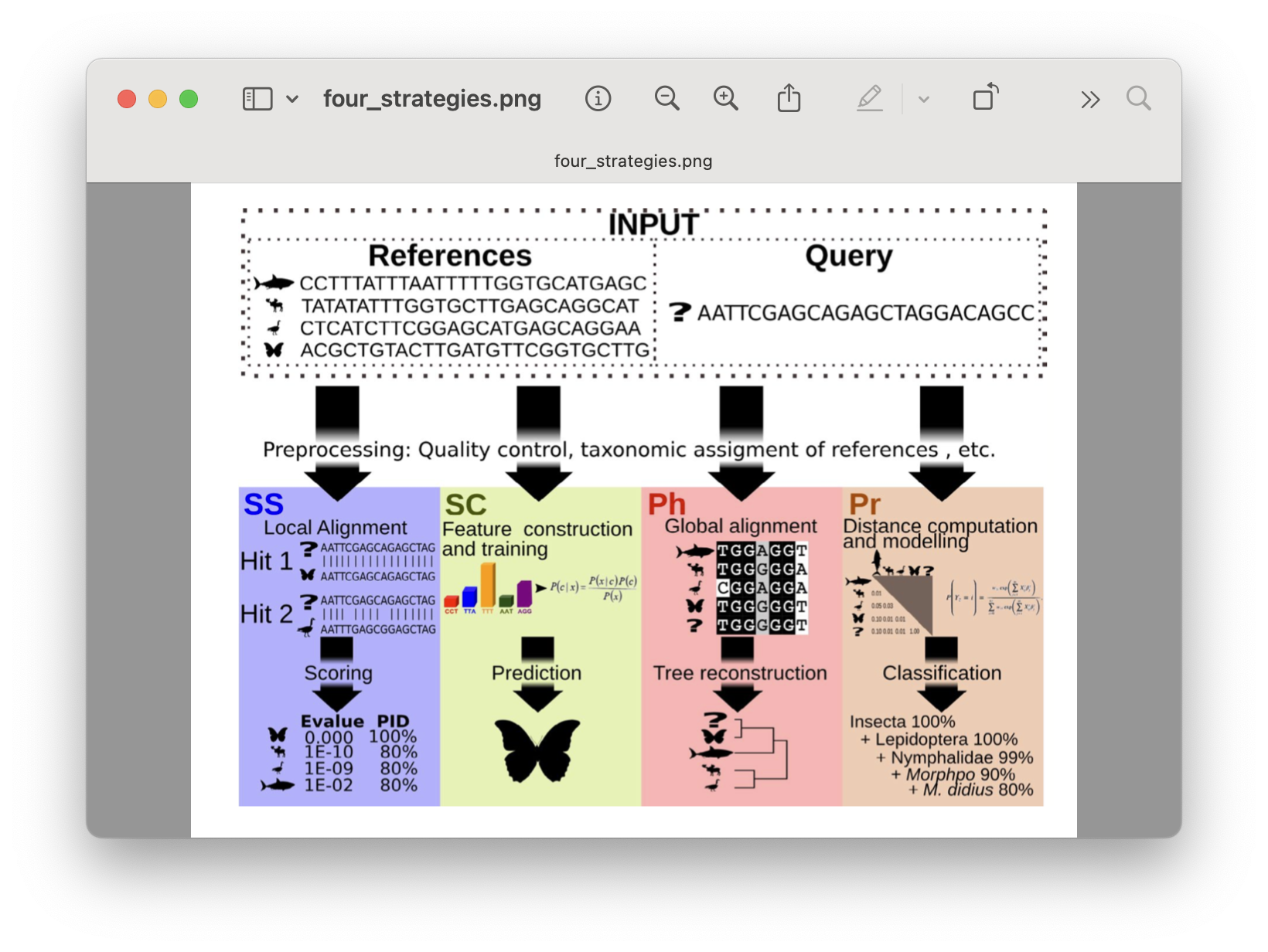
Fig. 29 : The four basic strategies to taxonomy classification. Copyright: Hleap et al., 2021#
Of the four abovementioned strategies to taxonomy classification, Sequency Similarity and Sequence Composition are most-frequently used in the metabarcoding research community. Multiple comparative experiments have been conducted to determine the most optimal approach to assign a taxonomic ID to metabarcoding data, though an optimal method is yet to be found. One example of a comparative study is the one from Bokulich et al., 2018.
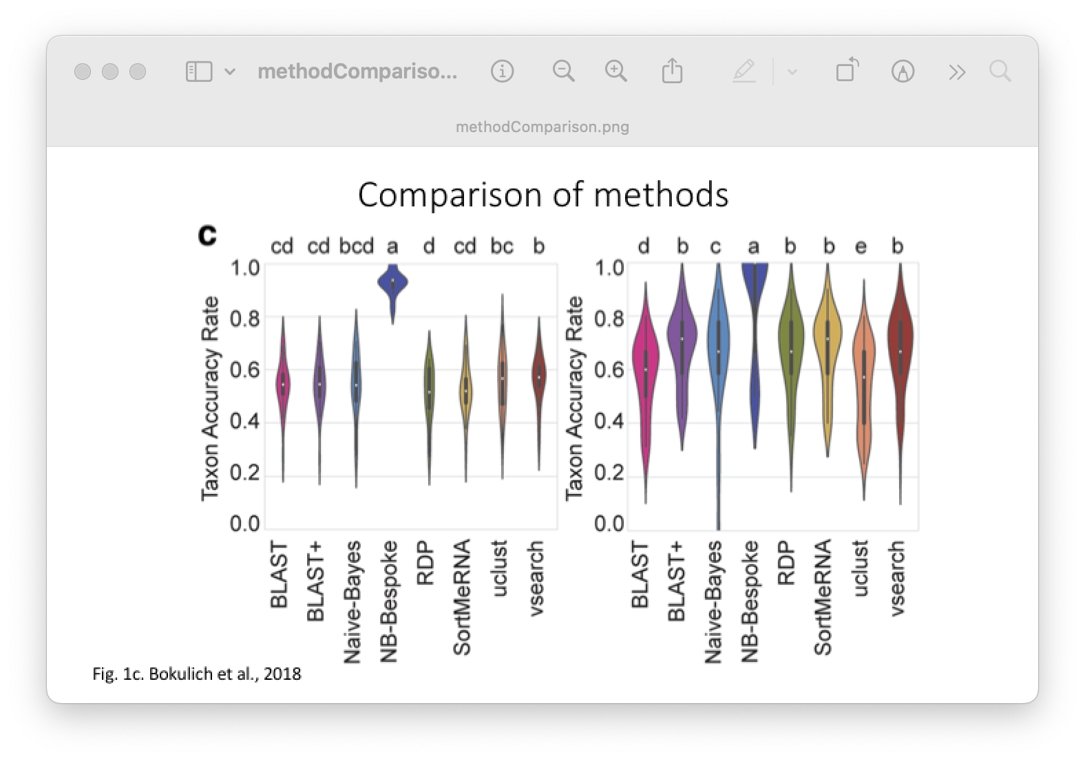
Fig. 30 : A comparison of taxonomy classifiers. Copyright: Bokulich et al., 2018#
While there are multiple ways to assign a taxonomic ID to a sequence, all methods require a reference database to match ASVs against a set of sequences with known taxonomic IDs. So, before we start with taxonomy assignment, let’s create our own local curated reference database using CRABS, which stands for Creating Reference databases for Amplicon-Based Sequencing. For more information on the sofware, I recommend reading the publication.
2. Online data repositories#
Several reference databases are available online. The most notable ones being NCBI, EMBL, BOLD, SILVA, and RDP. However, recent research has indicated a need to use custom curated reference databases to increase the accuracy of taxonomy assignment. While certain gene-specific or primer-specific reference databases are available (RDP: 16S microbial; MIDORI: COI eukaryotes; etc.), this essential data source is missing in most instances. We will, therefore, show you how to build your own custom curated reference database using CRABS.
Attention
Since the online COI reference material is quite large, it being the standard metazoan barcode gene, we will not build a COI reference database during this tutorial. Instead, we will use a pre-assembled COI database, which is already placed in your 5.refdb folder. However, to show you how to build your own database, we will go through the steps to build a 16S Chondrichthyes (sharks and rays) database, as the online reference material is small. Therefore, the steps can be accomplished quite quickly.
3. CRABS#
3.1 Workflow#
The current version of CRABS v1.7.7 includes 7 steps, namely:
download data from online repositories,
import downloaded data into CRABS format,
extract amplicons from imported data,
retrieve amplicons without primer-binding regions,
curate and subset the local database,
export the local database in various taxonomic classifier formats, and
basic visualisations to explore the local reference database.
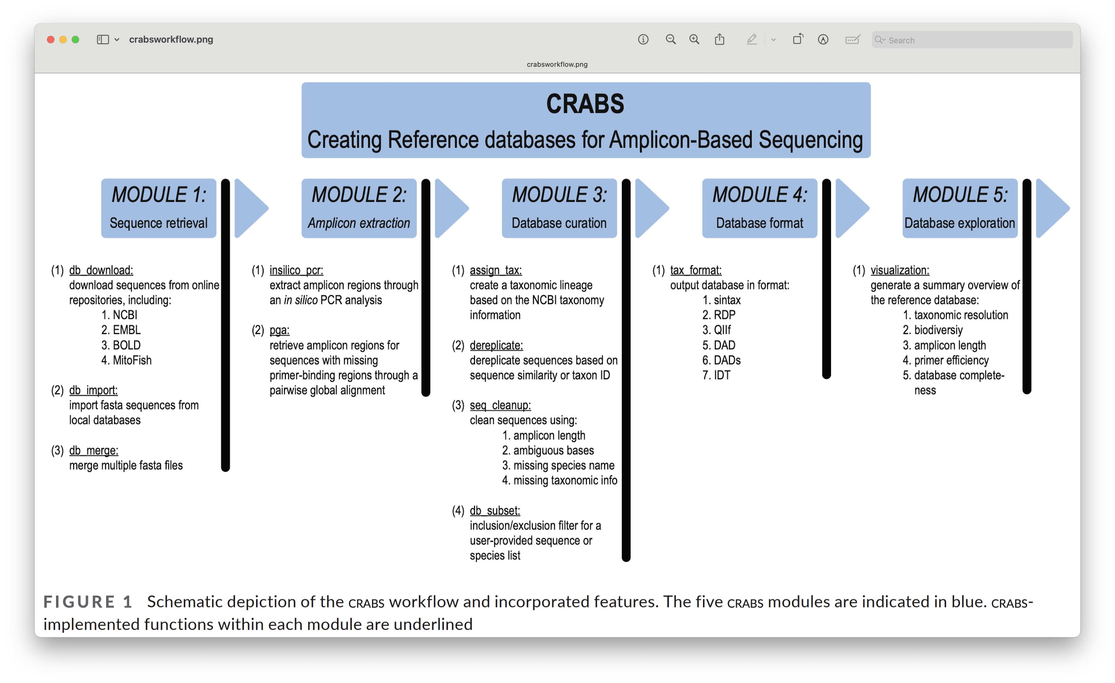
Fig. 31 : The CRABS workflow to create your own reference database. Copyright: Jeunen et al., 2023#
3.2 Help documentation#
To bring up the help documentation for CRABS, we can use the --help or -h command.
Running CLI programs in RStudio
CRABS is a CLI program written in Python, similar to cutadapt. However, rather than the system2() function we employed yesterday to run cutadapt, we will execute CRABS’ code into the Terminal window, rather than the Console window. For the remainder of this section, all code will be run in this fashion, unless stated otherwise.
So, let’s start RStudio and open a new text file, rather than an R script, and save it as taxonomy_assignment.txt in the bootcamp folder.
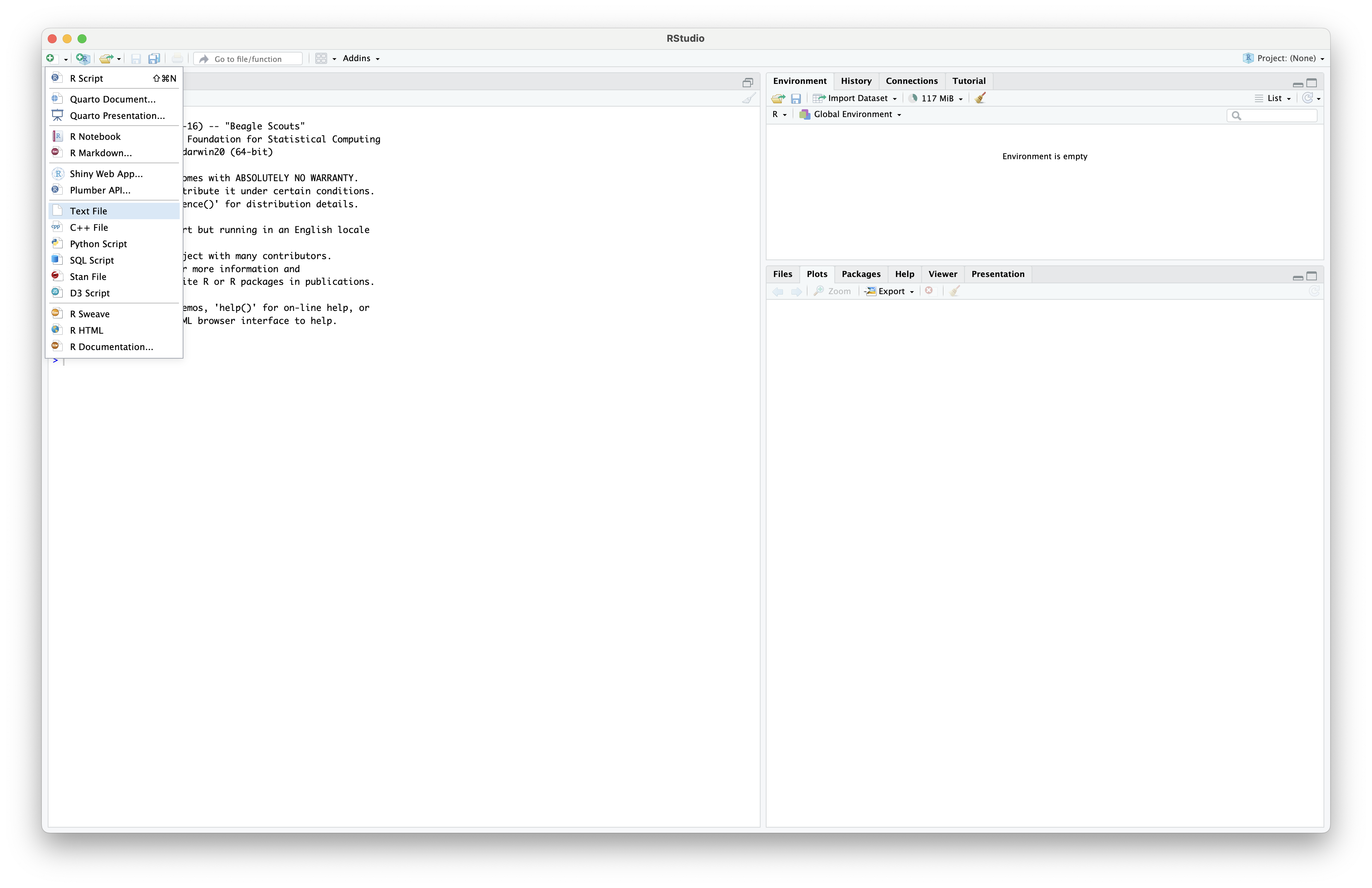
Fig. 32 : Opening up a text file in RStudio#
Now, let’s copy-paste the code to bring up the help documentation into the text file and run it in the Terminal window. You can run the code either by copy-pasting it in the Terminal window or by pressing command + option + return for MacOS and ctrl + alt + enter for Windows and Linux.
crabs -h
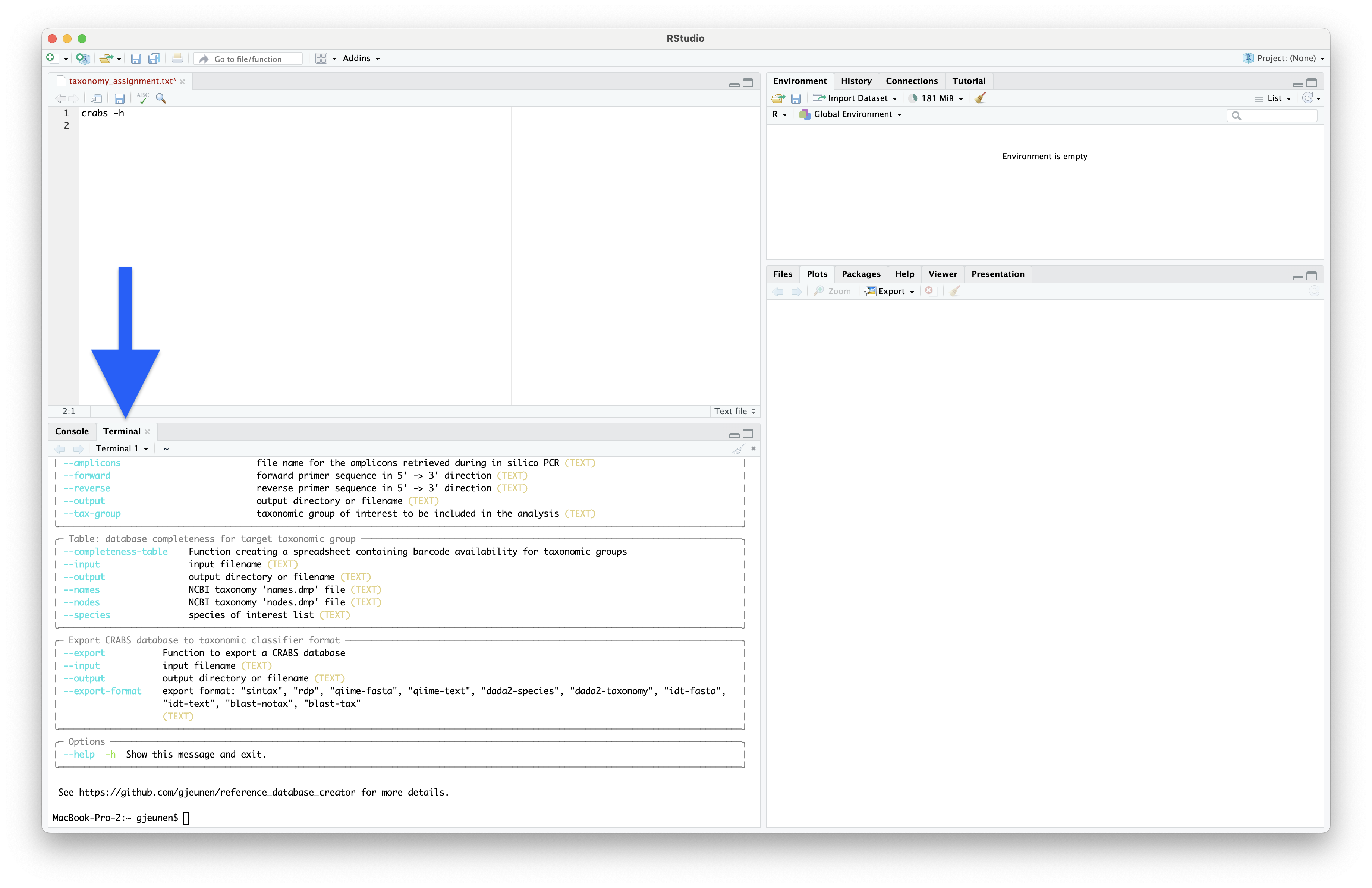
Fig. 33 : The CRABS help documentation#
3.3 Step 1: download data#
As a first step to create your local custom reference database, you will need to download data from online repositories or use barcode sequences that you have generated yourself. CRABS can download data from the 7 most widely-used online repositories, including BOLD, EMBL, GreenGenes, MIDORI2, MitoFish, NCBI, and SILVA.
For this tutorial, however, we will only focus on downloading shark sequences of the 16S gene from the NCBI online repository, as this database is the most widely-used in metabarcoding research, as well as the biggest online repository. To download data from the NCBI servers, we need to provide several parameters to CRABS. Maybe the trickiest to understand is the --query parameter. However, we can get the input string for this parameter from the NCBI website, as shown in the screenshot below.
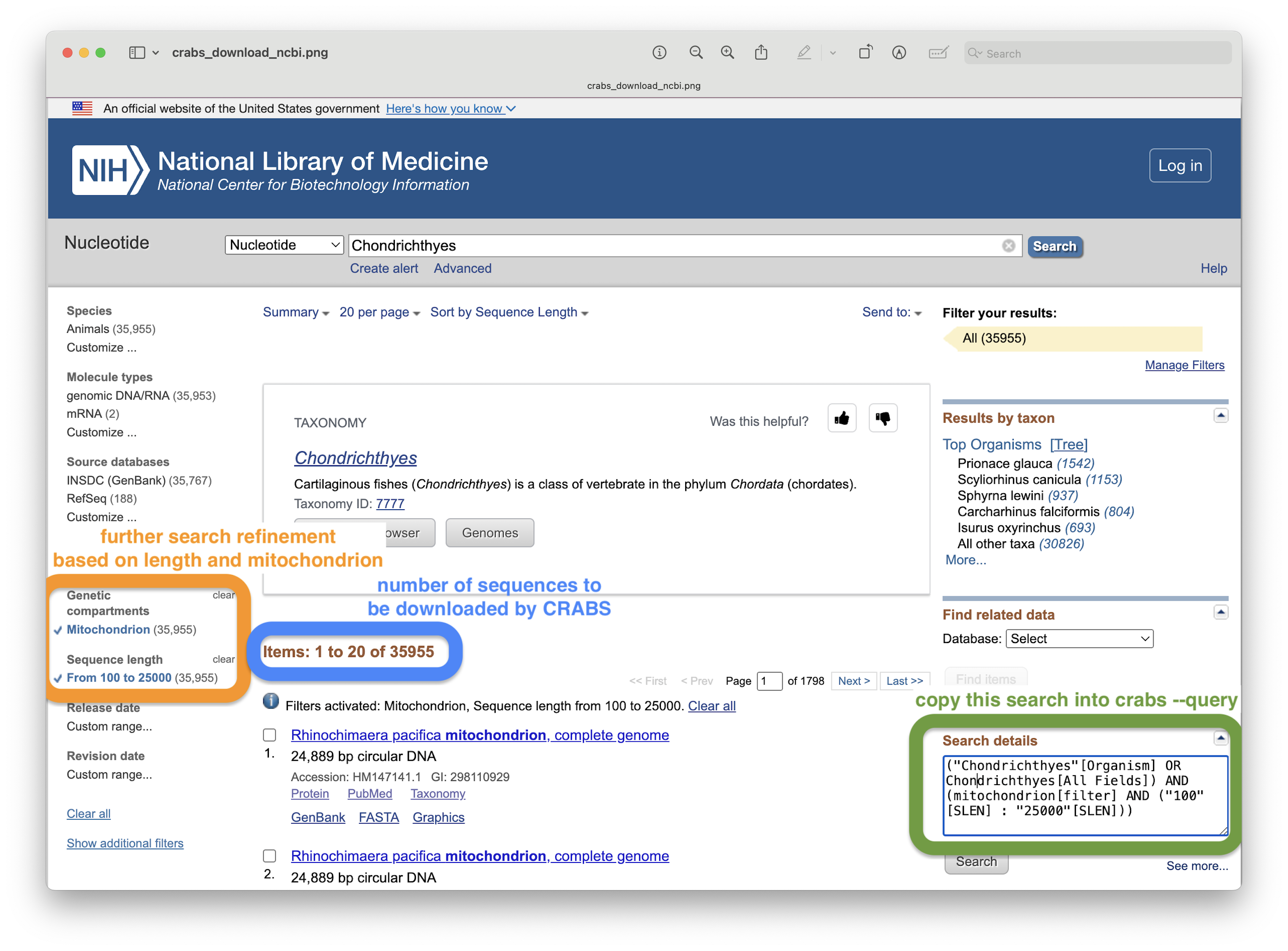
Fig. 34 : A screenshot of the NCBI website showing where to find the input value for the --query parameter#
Other parameters that are required are an output file name (--output), your email for identification by NCBI’s servers (--email), and the database you wish to download from (--database), which for metabarcoding data is usually nucleotide.
Before we can execute the code, we need to set our working directory. However, since we are working in the Terminal window, we need to provide slightly different commands, as this is not an R environment. To print the current working directory, we can use the pwd command. You should now see an output string in the Terminal window telling you the current working directory.
pwd
Output
/Users/gjeunen
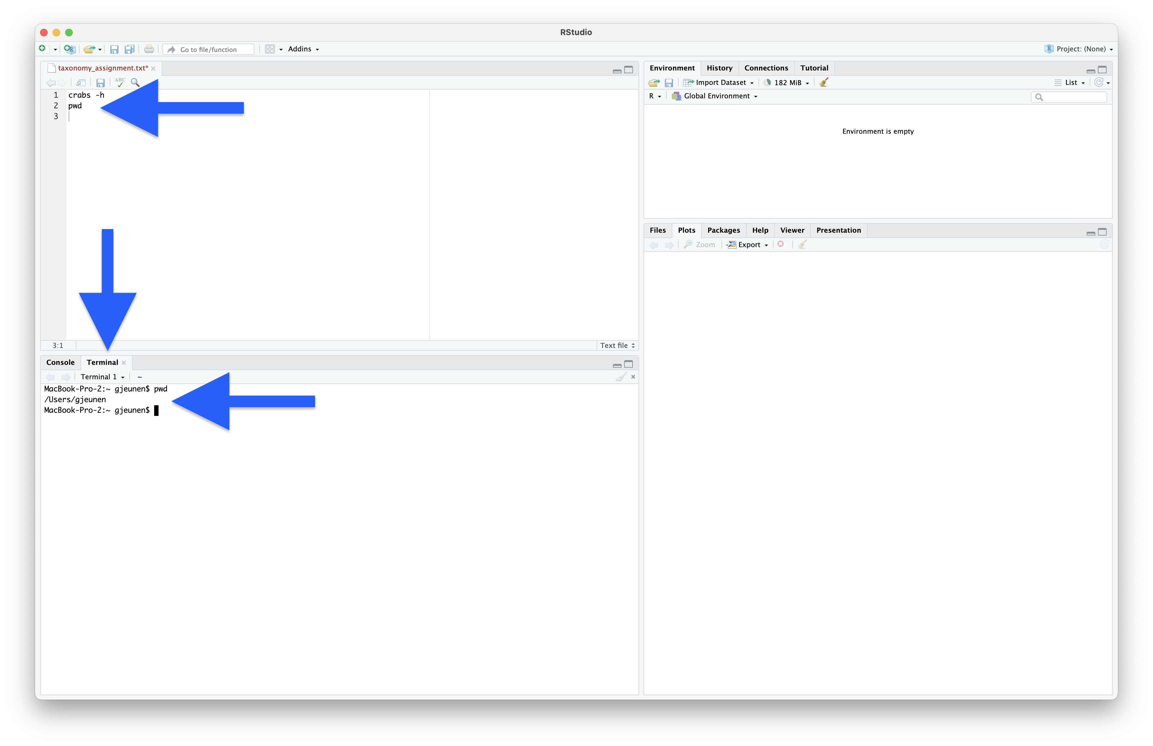
Fig. 35 : A screenshot of RStudio when running the pwd command in the Terminal window, executed by pressing command + option + return for MacOS or ctrl + alt + enter for Linux and Windows.#
To change the current working directory, we can use the cd command, which stands for change directory.
cd Desktop/bootcamp/5.refdb/
Navigating directories in the Terminal
The code above is for MacOS and Linux, slight alterations might be required for Windows users!
Now that we have navigated to the 5.refdb folder, let’s print the current working directory again to make sure we’re in the folder we expect.
pwd
Output
/Users/gjeunen/Desktop/bootcamp/5.refdb
We can also list the current files using the ls command, which stands for list. We can provide a couple of additional parameters to this command to format the output.
ls -ltr
Output
-rw-r--r--  1 gjeunen  staff    17850320 Apr  1 04:26 taxdb.bti
-rw-r--r--  1 gjeunen  staff   169532428 Apr  1 04:26 taxdb.btd
-rw-r--r--  1 gjeunen  staff    85700608 Apr  1 04:26 taxonomy4blast.sqlite3
-rw-r--r--  1 gjeunen  staff   201193865 Apr  2 19:26 nodes.dmp
-rw-r--r--  1 gjeunen  staff   265924736 Apr  2 19:27 names.dmp
-rw-r--r--  1 gjeunen  staff  1129185908 Apr  3 02:32 coi_clean.txt
-rw-r--r--  1 gjeunen  staff   207099442 Apr  3 03:15 coi_blast.nsq
-rw-r--r--  1 gjeunen  staff    10683728 Apr  3 03:15 coi_blast.nog
-rw-r--r--  1 gjeunen  staff    32051236 Apr  3 03:15 coi_blast.nin
-rw-r--r--  1 gjeunen  staff   158567715 Apr  3 03:15 coi_blast.nhr
-rw-r--r--  1 gjeunen  staff    12942204 Apr  3 03:15 coi_blast.nto
-rw-r--r--  1 gjeunen  staff    50335744 Apr  3 03:15 coi_blast.ntf
-rw-r--r--  1 gjeunen  staff    32051096 Apr  3 03:15 coi_blast.not
-rw-r--r--  1 gjeunen  staff    67982376 Apr  3 03:15 coi_blast.nos
-rw-r--r--  1 gjeunen  staff   132980736 Apr  3 03:15 coi_blast.ndb
-rw-r--r--  1 gjeunen  staff  2542038129 Apr  3 12:33 nucl_gb.accession2taxid.gz
You should see a list of 16 files, all related to the COI reference database we will be using later.
For now, let’s download the 16S shark barcodes from NCBI.
crabs --download-ncbi --query '(16S[All Fields] AND ("Chondrichthyes"[Organism] OR Chondrichthyes[All Fields])) AND mitochondrion[filter]' --email gjeunen@gmail.com --output ncbi_sharks.fasta --database nucleotide
Output
/// CRABS | v1.7.7

|            Function | Download NCBI database
|Retrieving NCBI info | ━━━━━━━━━━━━━━━━━━━━━━━━━━━━━━━━━━━━━━━━ 100% 0:00:00 0:00:00
|         Downloading | ━━━━━━━━━━━━━━━━━━━━━━━━━━━━━━━━━━━━━━━━ 100% 0:00:00 0:01:13
|             Results | Number of sequences downloaded: 3868/3868 (100.0%)
Let’s look at the top 10 lines of the output file to see what CRABS downloaded. We can use the head command for this and pass the -n 10 parameter to specify 10 lines.
head -n 10 ncbi_sharks.fasta
Output
>MZ562568.1 Fontitrygon garouaensis isolate GN19480 mitochondrion, partial genome
GCTAGCGTAGCTTAAACAAAAGCATAGCATTGAAGATGCTAAGATAAAAATTAACCTTTTTCGCAAGCAT
GAAGGTTTGGTCCTGGCCTCAATATTAGTTCTAACTTGATTTACACATGCAAGTCTCAGCATCCTGGTGA
GAACGCCCTACTTAAACCAAAAATTTAGACAGGAGCTGGTATCAGGTACACCATACAGGTAGCCCACAAC
ACCTCGCTCAGCCACACCCCCAAGGGAACTCAGCAGTGACTAACATTGTTCCATAAGCGTAAGCTTGAGC
CAATCAAAGTTAAGAGAGTTGGTTAATCTCGTGCCAGCCACCGCGGTTATACGAGTAACACAAATTAATA
TTTTACGGCGTTAAGGGTGATTAAAAATAAACTTCCCAAAAATAGAGTTAATACATCATCAAACCGTCAT
ACGTTTACATGCTCAAAAACATCACTCACGAAAGTAACTCTACATAAAAAAGACTTTTTGACCTCACGAT
AGTTAAGATCCAAACTAGGATTAGATACCCTATTATGCTTAACCATAAACATTGTCATAAAAATTTACCT
TAATATTACCGCCCGAGTACTACGAGCGCTAGCTTAAAACCCAAAGGACTTGGCGGTGCTCCAAACCCCC
From the output, we can see that CRABS has downloaded the original format from the NCBI servers, which in this case is a multi-line fasta document.
3.4 Step 2: import data#
Since CRABS can download data from multiple online repositories, each with their own format, we need to first reformat the data to CRABS format before we can continue building our reference database. This reformatting can be done using the --import function, which will create a single line text document for each sequence, that contains a unique ID, the taxonomic lineage for that sequence, plus the sequence itself. The CRABS taxonomic lineage is based on the NCBI taxonomy database and requires 3 files to be downloaded using the --download-taxonomy function. However, to speed things up, these 3 files have already been provided to you.
For those interested, you can download the three NCBI files using the following command (do not execute this command for the workshop, as the files are already in your folder!).
crabs --download-taxonomy
Before importing, we need to unzip one of the three taxonomy files, as it was too big to share (note: this won’t be necessary when downloading the files through CRABS).
gunzip nucl_gb.accession2taxid.gz
Once unzipped, we can import the downloaded NCBI data into CRABS format. To import data, we have to provide several parameters, including the format --import-format, the three taxonomy files (--names, --nodes, and --acc2tax), the input file (--input), an output file (--output), and optionally the taxonomic ranks to be included in the taxonomic lineage (--ranks).
crabs --import --import-format ncbi --names names.dmp --nodes nodes.dmp --acc2tax nucl_gb.accession2taxid --input ncbi_sharks.fasta --output ncbi_sharks.txt
Output
/// CRABS | v1.7.7

|            Function | Import sequence data into CRABS format
| Read data to memory | ━━━━━━━━━━━━━━━━━━━━━━━━━━━━━━━━━━━━━━━━ 100% 0:00:00 0:03:31
|Phylogenetic lineage | ━━━━━━━━━━━━━━━━━━━━━━━━━━━━━━━━━━━━━━━━ 100% 0:00:00 0:00:00
|Fill missing lineage | ━━━━━━━━━━━━━━━━━━━━━━━━━━━━━━━━━━━━━━━━ 100% 0:00:00 0:00:00
|             Results | Imported 3868 out of 3868 sequences into CRABS format (100.0%)
When we now look at the first line of the output file, we can see how CRABS has changed the structure from a multi-line fasta to a single line tab-delimited text file.
head -n 1 ncbi_sharks.txt
Output
MZ562568 Fontitrygon garouaensis 3355173 Metazoa Chordata Chondrichthyes Myliobatiformes Dasyatidae Fontitrygon Fontitrygon garouaensis GCTAGCGTAGCTTAAACAAAAGCATAGCATTGAAGATGCTAAGATAAAAATTAACCTTTTTCGCAAGCATGAAGGTTTGGTCCTGGCCTCAATATTAGTTCTAACTTGATTTACACATGCAAGTCTCAGCATCCTGGTGAGAA...
3.5 Step 3: extract amplicons through in silico PCR#
Once we have formatted the data, we can start with a first curation step of the reference database, i.e., extracting the amplicon sequences. We will be extracting the amplicon region from each sequence through an in silico PCR analysis. With this analysis, we will locate the forward and reverse primer binding regions and extract the sequence in between. This will significantly reduce file sizes when larger data sets are downloaded, while also ensuring that only the necessary information is kept.
We can use CRABS’ --in-silico-pcr function for this step, which requires us to provide information on the following parameters, the input file name (--input), the output file name (--output), the forward primer sequence (--forward), and the reverse primer sequence (--reverse). The primers for the 16S gene for which we are building a reference database are F: 5’-GACCCTATGGAGCTTTAGAC-3’ and R: 5’-CGCTGTTATCCCTADRGTAACT-3’. Note that we do not need to reverse complement the reverse primer when we provide this information to CRABS, who will do this for us before running the in silico PCR analysis.
crabs --in-silico-pcr --input ncbi_sharks.txt --output ncbi_sharks_amplicon.txt --forward GACCCTATGGAGCTTTAGAC --reverse CGCTGTTATCCCTADRGTAACT
Output
|  Transform to fasta | ━━━━━━━━━━━━━━━━━━━━━━━━━━━━━━━━━━━━━━━━ 100% 0:00:00 0:00:00
|       In silico PCR | ━━━━━━━━━━━━━━━━━━━━━━━━━━━━━━━━━━━━━━━━ 100% 0:00:00 0:00:00
|      Exporting data | ━━━━━━━━━━━━━━━━━━━━━━━━━━━━━━━━━━━━━━━━ 100% 0:00:00 0:00:00
|             Results | Extracted 3529 amplicons from 3868 sequences (91.24%)
From the output, we can see that we downloaded and imported 3,868 16S shark sequences from NCBI and CRABS managed to find the primer binding regions in 3,529 (91.24%) of them. So, nearly all.
3.6 Step 4: extract amplicons through pairwise global alignments#
Amplicons in the originally downloaded sequences might be missed during the in silico PCR analysis when one or both primer-binding regions are not incorporated in the online deposited sequence. This can happen when the reference barcode is generated with the same primer set or if the deposited sequence is incomplete in the primer-binding regions (denoted as “N” in the sequence). To retrieve those missed amplicons, we can use the already-retrieved amplicons as seed sequences in a Pairwise Global Alignment (PGA) analysis.
We can use CRABS’ --pairwise-global-alignment function for this step, which requires an input file name (--input), an amplicon file name (--amplicons), an output file name (--output), the forward (--forward) and reverse (--reverse) primer sequences, the minimum threshold value for the alignment similarity (--percent-identity), and the minimum threshold value for the alignment coverage of the amplicon (--coverage).
crabs --pairwise-global-alignment --input ncbi_sharks.txt --amplicons ncbi_sharks_amplicon.txt --output ncbi_sharks_pga.txt --forward GACCCTATGGAGCTTTAGAC --reverse CGCTGTTATCCCTADRGTAACT --percent-identity 0.9 --coverage 90
Output
/// CRABS | v1.7.7

|            Function | Retrieve amplicons without primer-binding regions
|         Import data | ━━━━━━━━━━━━━━━━━━━━━━━━━━━━━━━━━━━━━━━━ 100% 0:00:00 0:00:00
|  Transform to fasta | ━━━━━━━━━━━━━━━━━━━━━━━━━━━━━━━━━━━━━━━━ 100% 0:00:00 0:00:00
|  Pairwise alignment | ━━━━━━━━━━━━━━━━━━━━━━━━━━━━━━━━━━━━━━━━   0% -:--:-- 0:00:00
|             Results | Retrieved 42 amplicons without primer-binding regions from 339 sequences
The output shows us that by aligning the remaining sequences to the amplicons, we have retrieved another 42 amplicons for our reference database. The remaining 297 sequences we downloaded, albeit from the 16S gene region, are likely not covering at least 90% of the amplicon region of the 16S gene or are covering a different part of the 16S gene altogether.
3.7 Step 5: dereplicate the database#
Now that we have retrieved all amplicons from the downloaded sequences, we can remove duplicate sequences for each species, i.e., dereplicating the reference database. This step helps reduce the file size even more, plus is essential for most taxonomic classifiers that restrict the output to N number of best hits (such as the most widely used classifier BLAST).
To dereplicate the database, we can use CRABS’ --dereplicate function, which requires an input file name (--input) and an output file name (--output). By default, CRABS will retain all unique barcodes for each species, though you can change this to only keeping one barcode per species or only unique barcodes regardless if shared between different species using the --dereplication-method parameter.
crabs --dereplicate --input ncbi_sharks_pga.txt --output ncbi_sharks_derep.txt
Output
/// CRABS | v1.7.7

|            Function | Dereplicate CRABS database
|         Import data | ━━━━━━━━━━━━━━━━━━━━━━━━━━━━━━━━━━━━━━━━ 100% 0:00:00 0:00:00
|      Exporting data | ━━━━━━━━━━━━━━━━━━━━━━━━━━━━━━━━━━━━━━━━ 100% 0:00:00 0:00:00
|             Results | Written 746 unique sequences to ncbi_sharks_derep.txt out of 3571 initial sequences (20.89%)
The output shows us that a lot of duplicate data was in our database and that we can reduce the reference database by 79.11% without losing any information.
3.8 Step 6: filter the reference database#
The final curation step for our custom reference database is to clean up the database using a variety of parameters, including minimum length, maximum length, maximum number of ambiguous base calls, environmental sequences, sequences for which the species name is not provided, and sequences with unspecified taxonomic levels. To accomplish this, we can use the --filter function, for which we need to provide an input file name (--input), an output file name (--output), and values for the different parameters.
crabs --filter --input ncbi_sharks_derep.txt --output ncbi_sharks_clean.txt --minimum-length 150 --maximum-length 250 --environmental --no-species-id --maximum-n 1 --rank-na 2
Output
/// CRABS | v1.7.7

|            Function | Filter CRABS database
| Included parameters | "--minimum-length", "--maximum-length", "--maximum-n", "--environmental", "--no-species-id", "--rank-na"
|         Import data | ━━━━━━━━━━━━━━━━━━━━━━━━━━━━━━━━━━━━━━━━ 100% 0:00:00 0:00:00
|      Exporting data | ━━━━━━━━━━━━━━━━━━━━━━━━━━━━━━━━━━━━━━━━ 100% 0:00:00 0:00:00
|             Results | Written 728 filtered sequences to ncbi_sharks_clean.txt out of 746 initial sequences (97.59%)
|                     | Maximum ambiguous bases filter: 18 sequences not passing filter (2.41%)
The output shows that we only discarded 18 sequences, which contained too many ambiguous bases in the barcode sequence. These ambiguous bases are likely originating from unclean Sanger sequencing outputs, where a high confidence basecall cannot be made.
3.9 Step 7: export the reference database#
Now that we have created a custom curated reference database containing 728 shark sequences for the 16S rRNA gene in 6 simple steps, all that is left to do is to export the database in a format that can be used by a taxonomic classifier. As mentioned before, a huge variety of taxonomic classifiers exists, each requiring their own specific file format. Luckily, CRABS is capable of exporting your custom reference database to multiple taxonomic classifiers, including SINTAX, RDP, QIIME, DADA2, IDTAXA, and BLAST.
To show you how this works, we will export the current shark database to SINTAX format, which is a kmer based classifier implemented in USEARCH and VSEARCH. This requires the --export function in CRABS and needs an input file name (--input), an output file name (--output), and the format in which the database needs to be exported (--export-format).
crabs --export --input ncbi_sharks_clean.txt --output ncbi_sharks_sintax.fasta --export-format sintax
Output
/// CRABS | v1.7.7

|            Function | Export CRABS database to SINTAX format
|         Import data | ━━━━━━━━━━━━━━━━━━━━━━━━━━━━━━━━━━━━━━━━ 100% 0:00:00 0:00:00
|      Exporting data | ━━━━━━━━━━━━━━━━━━━━━━━━━━━━━━━━━━━━━━━━ 100% 0:00:00 0:00:00
|             Results | Written 728 sequences to ncbi_sharks_sintax.fasta out of 728 initial sequences (100.0%)
We can now have a look at the first 2 lines of the newly-created document to see what the SINTAX format looks like.
head -n 2 ncbi_sharks_sintax.fasta
Output
>MZ562568;tax=d:Metazoa,p:Chordata,c:Chondrichthyes,o:Myliobatiformes,f:Dasyatidae,g:Fontitrygon,s:Fontitrygon_garouaensis
ACTTAAATTATTTCTAACCAAACTCCTACCTCCGGGCATAAACCAAAAAAGAATCTTAATTTAACCTGTTTTTGGTTGGGGCGACCAAGGGGAAAAATAAAACCCCCTTATCGAACGTGTGAACAGTCACTCAAAAATTAGAACTACCACTCTAATTAATAGAAAATCTAACGAATAATGACCCAGGAATACATTTCCTGATCATTGGACCA
The SINTAX format is a 2-line fasta document, with the header on the first line containing the full taxonomic lineage of the barcode, and the sequence on the second line.
That’s all that it takes to generate your own reference database. We are now ready to assign a taxonomy to our ASVs that were generated during the bioinformatic pipeline in the previous section!
4. The COI reference database#
For our tutorial dataset, we will be using a COI reference database I generated earlier using CRABS (coi_blast). This database was generated using COI barcodes from NCBI, BOLD, and MIRODI2, as well as supplemented by local barcodes provided by students of this class. This reference database is formatted according to BLAST specifications and holds 2,670,924 high quality, unique, COI reference barcodes. In case you are interested, we have also provided you the unformatted COI reference database in CRABS format (coi_clean.txt), if you’d like to export the database in a different format and trial other taxonomic classifiers for this dataset or your own data.
5. BLAST#
5.1 Online BLAST#
The taxonomic classifier we will be using for this tutorial is BLAST (Basic Local Alignment Search Tool). BLAST is probably the most well-known classifier, as well as the most widely used one. As the name suggests, BLAST assigns a taxonomic ID to a sequence through best hits from local alignments against a reference database. Hence, when thinking about the four basic strategies for taxonomy assignment we introduced earlier, BLAST belongs to the Sequence Similarity (SS) category.
The popularity of BLAST likely stems from its direct implementation into the NCBI online reference database repository. To check out the website, we will copy-paste the first 5 sequences in our ASV file (4.results/asvs.fasta) and perform a Nucleotide BLAST, as shown in the screenshot below.
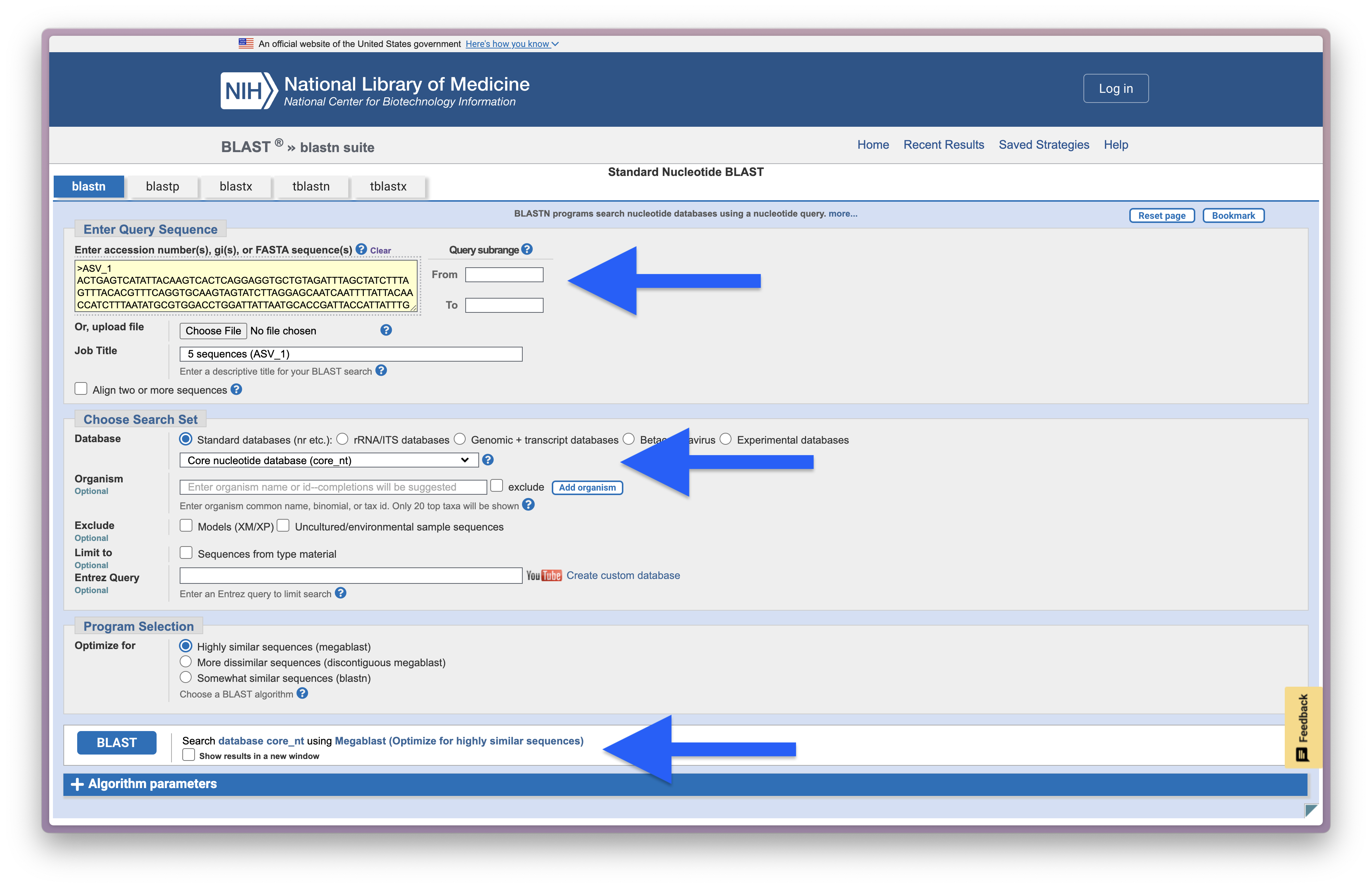
Fig. 36 : A screenshot of the setup for an online BLAST search#
And below is a screenshot of the BLAST results for ASV_1.
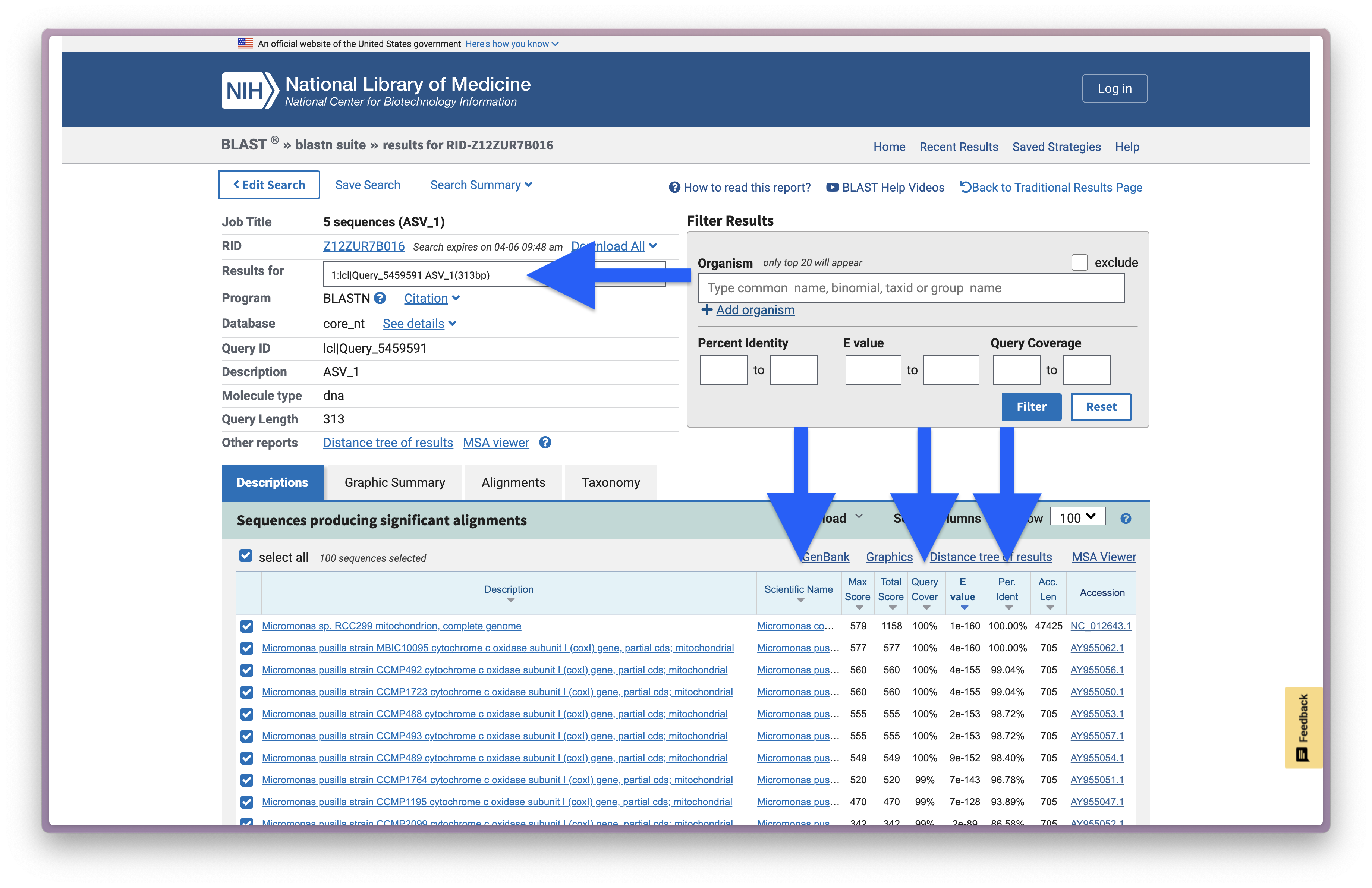
Fig. 37 : A screenshot of the online BLAST results for ASV_1#
We will explore the results on the website more in depth during the workshop, but the most important numbers are provided in the screenshot above, including the ASV ID (Results for), the taxonomic ID the sequence best matches to (Scientific Name), the percentage of how much the reference sequence provides coverage to the query sequence (Query Cover), the expected value is a parameter that describes the number of hits one can “expect” to see by chance when searching a database of a particular size and describes the random background noise (E value), and the percent identity value of how well the query and reference match over the covered region (Per. Ident).
5.2 Local BLAST#
While the website is extremely handy, it will be time-consuming if we have to check all 8,314 ASVs in our 4.results/asvs.fasta file. Plus, besides being time-consuming, the NCBI servers also limit the number of sequences you can BLAST per time and might restrict server access if you are taking up too much bandwidth. Luckily, BLAST is also available via the Command Line Interface, called BLAST+, and can be run locally on curated reference databases without restrictions. Furthermore, since CRABS can download data from multiple online repositories, as well as incorporate in house barcodes, running BLAST locally will aid in increased taxonomic assignment accuracy by incorporating a larger number of barcodes.
When we conduct BLAST via the command line (function: blastn), we can specify that we want to search against the custom local reference database by specifying the local database name to the -db parameter. Our query sequences are provided through the -query parameter. We can also set the maximum number of target sequences we get back, the minimum percent identity threshold, and the minimum query coverage threshold through the -max_target_seqs, -perc_identity, and -qcov_hsp_perc parameters. Finally, the output file (parameter -out) can take on different formats, but the most common is a tab-delimited structure, which is invoked by -outfmt "6". Table C1 in this document provides an overview of all the different options to the BLAST+ search application.
blastn -db coi_blast -query ../4.results/asvs.fasta -out ../4.results/blast_results.txt -max_target_seqs 50 -perc_identity 50 -qcov_hsp_perc 50 -outfmt "6 qaccver saccver staxid sscinames length pident mismatch qcovs evalue bitscore qstart qend sstart send gapopen"
We can inspect the BLAST output using the head command.
head -n 10 ../4.results/blast_results.txt
Output
ASV_1   FJ859351        296587  Micromonas commoda      313     100.000 0       100     9.88e-164       579     1       313     1   313      0
ASV_1   AY955062        38833   Micromonas pusilla      312     100.000 0       99      3.55e-163       577     2       313     1   312      0
ASV_1   AY955050        38833   Micromonas pusilla      312     99.038  3       99      3.58e-158       560     2       313     1   312      0
ASV_1   AY955056        38833   Micromonas pusilla      312     99.038  3       99      3.58e-158       560     2       313     1   312      0
ASV_1   AY955053        38833   Micromonas pusilla      312     98.718  4       99      1.66e-156       555     2       313     1   312      0
ASV_1   AY955057        38833   Micromonas pusilla      312     98.718  4       99      1.66e-156       555     2       313     1   312      0
ASV_1   AY955054        38833   Micromonas pusilla      312     98.397  5       99      7.74e-155       549     2       313     1   312      0
ASV_1   AY955060        38833   Micromonas pusilla      311     96.785  10      99      6.07e-146       520     3       313     2   312      0
ASV_1   AY955063        38833   Micromonas pusilla      311     93.891  19      99      6.20e-131       470     2       312     1   311      0
ASV_1   AY955052        38833   Micromonas pusilla      313     86.581  38      99      1.41e-92        342     2       312     1   311      4
From the output, we can see that we have a tab-delimited text file with the same number of columns provided as the argument we passed to the -outfmt parameter for the blastn function. The most important columns to note are the first one representing the ASV ID, the second column representing the reference barcode ID, the fourth column representing the species ID of the reference barcode, the sixth column representing the percent similarity of the alignment between our ASV and the reference barcode, and the eight column representing the coverage of the amplicon over which the alignment spans. We can also see that we have a multiple hits per ASV, each above the similarity and coverage threshold of 50 (as specified by -perc_identity and -qcov_hsp_perc), and with a maximum of 50 hits as specified by the -max_target_seqs parameter.
5.3 BLAST output parsing#
One of the last things needed to finalise taxonomy assignment for our ASVs after receiving the BLAST results, is to parse the output file. Currently, we have an output file with potentially mutliple BLAST hits, that could have identical or differing percent identity and query coverage values, as well as be assigned to the same species or different species.
A frequently-used approach to parse BLAST outputs is to calculate the Most Recent Common Ancestor or MRCA. Today, we will be using a small script I have created that takes in a BLAST output file, finds the MRCA among all hits per ASV, creates the taxonomic lineage for the MRCA, and, finally, provides the list of matching species ID’s that was used to create the MRCA. To accomplish this, we will be using the --mrca function of ALEX (Ancestor Link EXplorer), which requires us to provide the blast input file (--blast-input), the count table (--table-input) so that ALEX can write the MRCA results in the same order and facilitate import into R downstream, as well as the names.dmp (--names-input) and nodes.dmp (--nodes-input) NCBI taxonomy files to create the taxonomic lineage. Finally, we need to provide an output file name using the --output parameter. Those two files are already in our 5.refdb folder, as we used them for CRABS as well. However, if you want to download them separately, you can do so through ALEX as well via the --download-taxonomy function.
alex --mrca --blast-input ../4.results/blast_results.txt --table-input ../4.results/count_table.txt --names-input names.dmp --nodes-input nodes.dmp --output ../4.results/blast_parsed.txt
Output
/// ALEX | v0.1.0

|            Function | Calculate MRCA from BLAST result
|       Extracting... | ━━━━━━━━━━━━━━━━━━━━━━━━━━━━━━━━━━━━━━━━ 100% 0:00:00 0:00:00
|       Extracting... | ━━━━━━━━━━━━━━━━━━━━━━━━━━━━━━━━━━━━━━━━ 100% 0:00:00 0:00:00
|       Extracting... | ━━━━━━━━━━━━━━━━━━━━━━━━━━━━━━━━━━━━━━━━ 100% 0:00:00 0:00:00
|       Extracting... | ━━━━━━━━━━━━━━━━━━━━━━━━━━━━━━━━━━━━━━━━ 100% 0:00:00 0:00:03
|       Extracting... | ━━━━━━━━━━━━━━━━━━━━━━━━━━━━━━━━━━━━━━━━ 100% 0:00:00 0:00:04
|       Extracting... | ━━━━━━━━━━━━━━━━━━━━━━━━━━━━━━━━━━━━━━━━ 100% 0:00:00 0:00:00
|       Extracting... | ━━━━━━━━━━━━━━━━━━━━━━━━━━━━━━━━━━━━━━━━ 100% 0:00:00 0:00:00
|       Extracting... | ━━━━━━━━━━━━━━━━━━━━━━━━━━━━━━━━━━━━━━━━ 100% 0:00:00 0:00:00
Finally, let’s use the head command once more to inspect the parsed results. We will print out the first 5 ASVs, so that we can compare them to the online BLAST results.
head -n 10 ../4.results/blast_parsed.txt
Output
#OTU ID kingdom phylum  class   order   family  genus   species pident  qcov    matching species IDs
ASV_1   Viridiplantae   Chlorophyta     Mamiellophyceae Mamiellales     Mamiellaceae    Micromonas      NA      100.0   100     Micromonas commoda
ASV_2   Viridiplantae   Chlorophyta     Mamiellophyceae Mamiellales     Mamiellaceae    Micromonas      Micromonas_pusilla      100.099      Micromonas pusilla
ASV_3   Metazoa Arthropoda      Insecta Diptera Lonchaeidae     Lonchaea        Lonchaea_fraxina        78.966  90      Lonchaea fraxina
ASV_4   Viridiplantae   Chlorophyta     Mamiellophyceae Mamiellales     Mamiellaceae    Micromonas      Micromonas_pusilla      100.099      Micromonas pusilla
ASV_5   NA      NA      Phaeophyceae    Dictyotales     Dictyotaceae    Canistrocarpus  Canistrocarpus_crispatus        82.253  93  Canistrocarpus crispatus
That’s it for creating your own local reference database and taxonomy assignment. Next up is data curation, followed by the generation of phylogenetic trees, and statistical analysis of metabarcoding data!