Japan eDNA bootcamp 2025

Welcome to the environmental DNA (eDNA) bootcamp held at the University of the Ryukyus!

The primary goal of this course is to introduce you to the analysis of metabarcoding sequence data, with a specific focus on environmental DNA or eDNA, and ultimately make you comfortable to explore your own next-generation sequencing data. The sessions are split up into three days, with the bioinformatic analysis on Wednesday 16 April, taxonomic assignment and data curation on Thursday 17 April, and statistical analysis and visualisations on Friday 18 April. At the end of the three days, we hope you will be able to understand and execute the main steps in a bioinformatic pipeline, build your own custom reference database, assign a taxonomic ID to your sequences using different algorithms, further curate your data, and analyse data in a statistically correct manner.

1. Introduction

Based on yesterday’s excellent presentations, we can get an understanding of how broadly applicable eDNA metabarcoding is and how many research fields are using this technology to answer ecological questions.

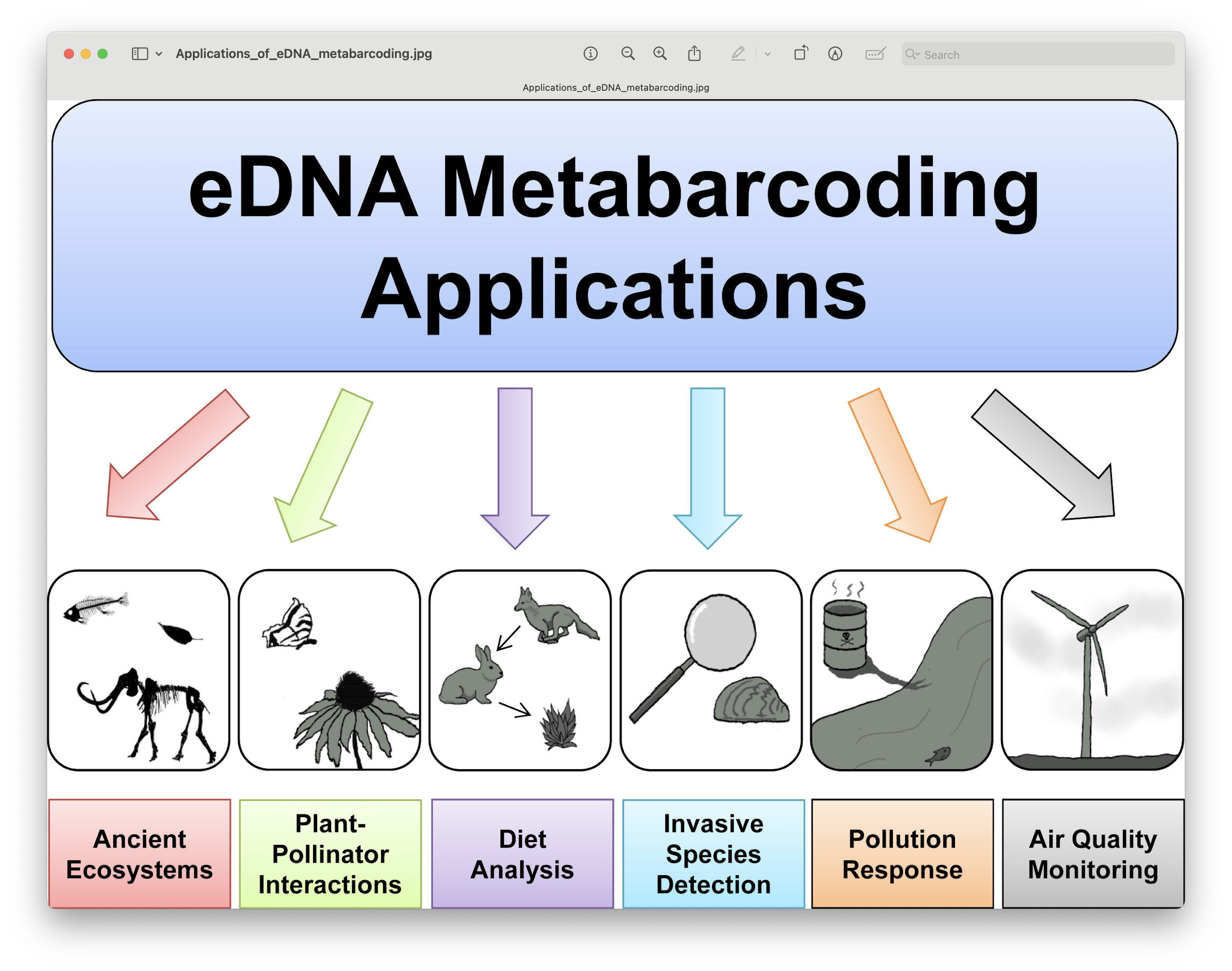
Fig. 1 : a general overview of the different applications of eDNA metabarcoding research.

Before we get started with coding, we will first introduce the data we will be analysing, some of the software programs available (including the ones we will use in this bootcamp), and the general structure of a bioinformatic pipeline to process metabarcoding data. Finally, we will go over the folder structure we suggest you use during the processing of metabarcoding data to help keep an overview of the files and ensure reproducibility of the analysis.

2. Experimental setup

The data we will be analyzing is part of a larger eDNA metabarcoding project jointly conducted by the team of Prof. James Reimer, Molecular Invertebrate Systematics and Ecology Laboratory (MISE, University of the Ryukyus) and Prof. Timothy Ravasi, Marine Climate Change Unit (Okinawa Institute of Science and Technology; OIST). One of the goals of this collaborative research is to examine how fish community composition changes across a latitudinal gradient in Japan, with a particular interest in assessing evidence for tropicalization—i.e., the poleward spread of tropical species due to ocean warming.

To investigate this, surface seawater samples were collected from various sites throughout Japan, ranging from temperate to subtropical regions. Samples were taken either from boats or directly from manmade structures such as seawalls and harbors. At each site, three replicate 2-liter surface water samples were collected using a sterilized bucket and transferred into sterile Mighty Bags (Maruemu Corp., Osaka, Japan). To account for potential contamination during sampling and processing, two controls were included per sampling day. A field control was prepared by opening a bottle of sterile water for five minutes at the sampling location, while a filter control was done using the same procedure immediately prior to filtration.

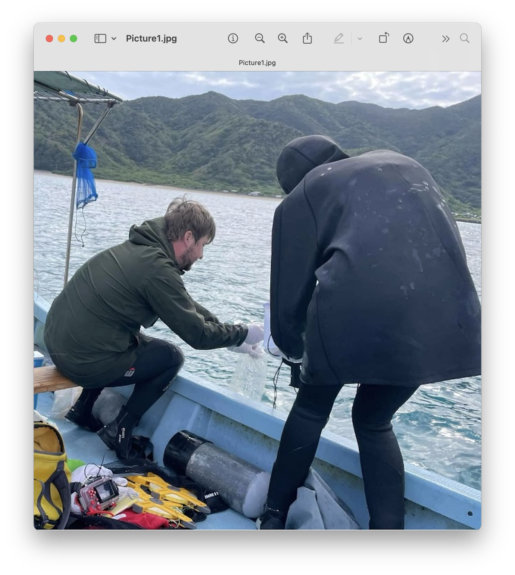
Fig. 2 : eDNA water sample collection Amami-Oshima, November 2022

Water samples and field controls were filtered using 0.45 µm Sterivex filters (Merck, Darmstadt, Germany) using an Aspirator (As One, Osaka, Japan). Filters were preserved in RNAlater (Sigma-Aldrich, St. Louis, USA) and stored at –80°C until extraction. DNA was extracted following a modified protocol based on the Qiagen DNeasy Blood & Tissue Kit (Açıkbaş et al., 2024). Metabarcoding was carried out using a ~313 bp fragment of the mitochondrial cytochrome c oxidase subunit I (COI) gene, using primers and protocols described by Leray et al. (2013). The resulting data will be used to evaluate spatial biodiversity patterns along Japan’s coastline.

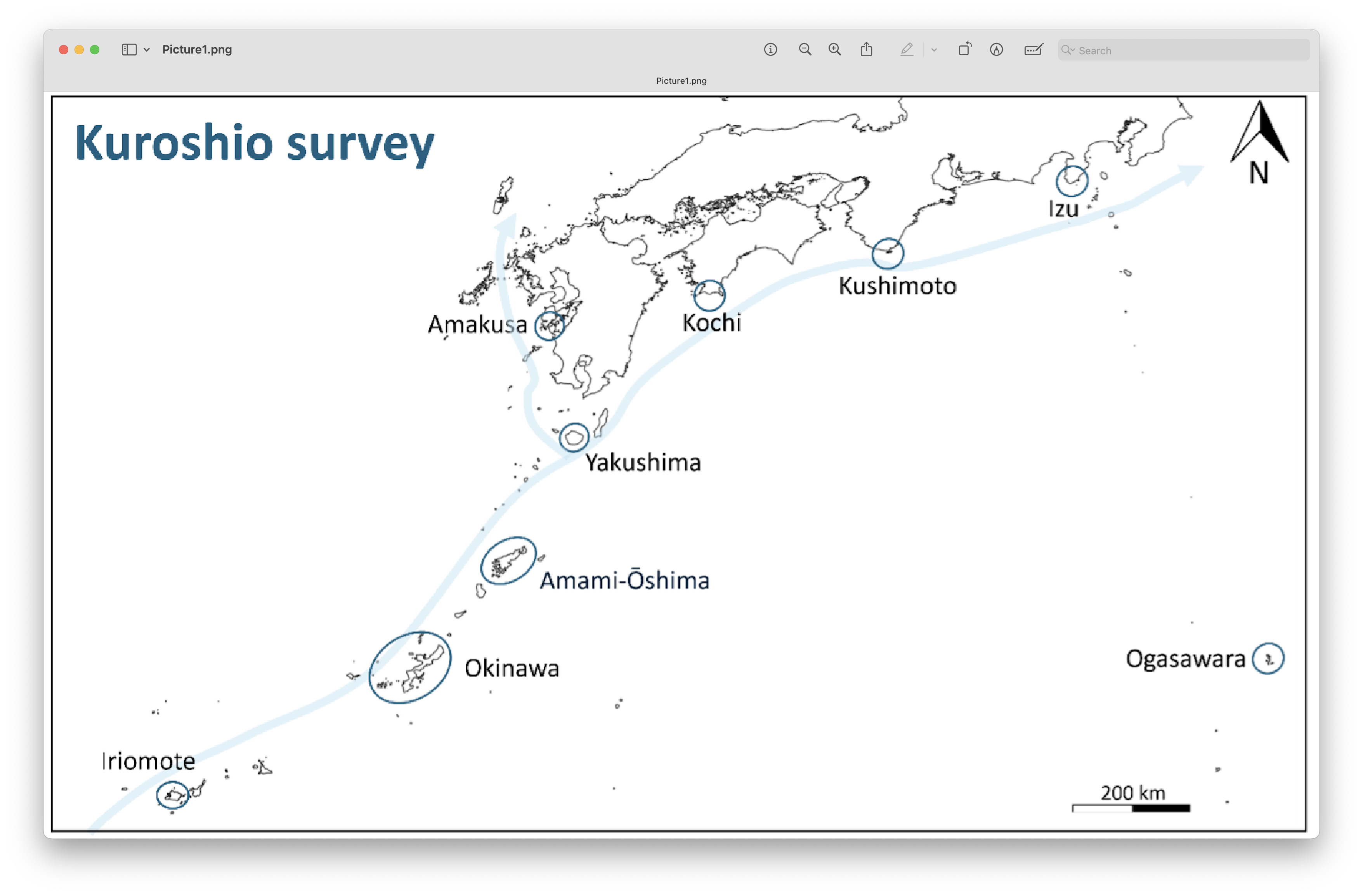
Fig. 3 : Sampling locations in Japan

The subset of samples we will be working with during the workshop were collected during a research trip to Amami-Oshima in November 2022. This expedition was initiated by Megumi Nakano (then with the Nature Conservation Society of Japan) in response to concerns raised by local island residents regarding perceived changes in their surrounding reef ecosystems. The trip aimed to document current biodiversity patterns and provide baseline data that could help assess potential shifts in reef community composition.

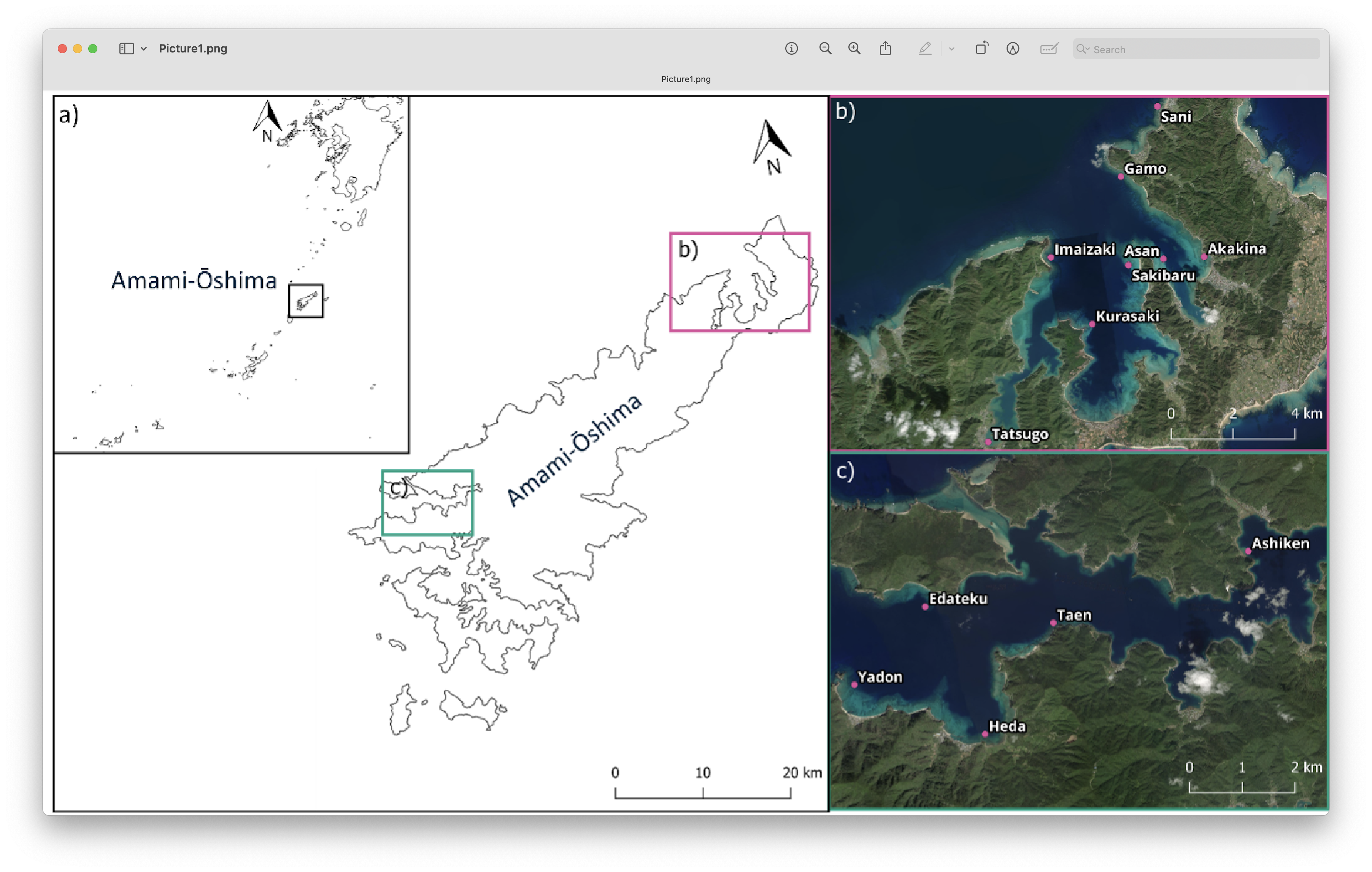
Fig. 4 : Sampling locations Amami-Ōshima. a) Location of Amami-Ōshima in the island chains of the Ryukyus. b,c) Sample locations of eDNA water samples on Amami-Ōshima

3. A note on software programs

The popularity of metabarcoding research, both in the bacterial and eukaryote kingdom, has resulted in the development of a myriad of software packages and pipelines. Furthermore, software packages are continuously updated with new features, as well as novel software programs being designed and published. We will be using several software programs and R packages during this bootcamp. However, we would like to stress that the pipeline used in the workshop is by no means better than other pipelines and we urge you to explore alternative software programs and trial them with your own data after this workshop.

Metabarcoding software programs can generally be split up into two categories, including:

1. stand-alone programs that are self-contained: These programs usually incorporate novel functions or alterations on already-existing functions. Programs can be developed for a specific task within the bioinformatic pipeline or can execute multiple or all steps in the bioinformatic pipeline. Examples of such programs are: Mothur, USEARCH, VSEARCH, cutadapt, dada2, OBITools3.

2. wrappers around existing software: These programs attempt to provide an ecosystem for the user to complete all steps within the bioinformatic pipeline without needing to reformat documents or change the coding language. Examples of such programs are: QIIME2 and JAMP.

Below, we can find a list of some of the software programs and R packages that are available for analysing metabarcoding data (those marked with a ‘*’ will be covered in this workshop; please note that this list is not exhaustive and many other programs are available):

1. Bioinformatic processing:

   1. FASTQC: assess quality of .fastq files.

   2. MULTIQC: concatenate FastQC reports to enable comparisons between samples.

   3. cutadapt*: remove adapter regions from sequence data.

   4. VSEARCH: bioinformatic processing of metabarcoding data.

   5. dada2*: bioinformatic processing of metabarcoding data in R.

   6. Qiime2: a collection of different programs and packages, all compiled into a single ecosystem for bioinformatic analysis.

   7. Mothur: one of the first software programs to analyse metabarcoding data.

   8. JAMP: Just Another Metabarcoding Pipeline in R.

2. Taxonomy assignment:

   1. CRABS*: build custom curated reference databases.

   2. SINTAX: k-mer based classifier to assign a taxonomic ID to sequences.

   3. IDTAXA (RStudio): machine learning classifier to assign a taxonomic ID to sequences.

   4. BLAST*: local alignment classifier to assign a taxonomic ID to sequences.

   5. BOLDigger3: a Python program to query .fasta files against the BOLD V5 databases.

3. Data curation:

   1. tombRaider*: an algorithm to identify artefacts from metabarcoding data.

   2. LULU: an R-package for distribution-based post clustering curation of amplicon data.

   3. microDecon: an R-package for removing contamination from metabarcoding datasets post-sequencing.

   4. Decontam: an R-package for identifying contaminants in marker-gene and metagenomics data.

4. Statistical analysis:

   1. Phyloseq: R package to explore metabarcoding data.

   2. iNEXT.3D: R package to calculate inter- and extrapolation of alpha diversity measures.

   3. ape: R package to build multiple sequence alignments and phylogenetic trees.

   4. microbiome: R package as an extension to phyloseq.

   5. indicspecies: R package to calculate indicator species values

   6. vegan: R package to calculate various alpha and beta diversity measures.

   7. ggtree: build phylogenetic tree graphics.

Warning

Some software programs change the standard structure of your file to be compatible with the functions implemented within the program. When implementing several software programs in your bioinformatic pipeline, such modifications in the file structure could lead to incompatability issues when switching to the next program in your pipeline. It is, therefore, important to understand how a specific program changes the structure of the sequence file and learn how these modifications can be reverted back (through simple python, bash, or R scripts). We will talk a little bit more about file structure and conversion over the coming days.

In a recent meta-analysis our lab conducted, which included ~600 scientific publications on metabarcoding from 2023, we can see that dada2 and USEARCH-VSEARCH are the most prominently-used software programs in the metabarcoding research community.

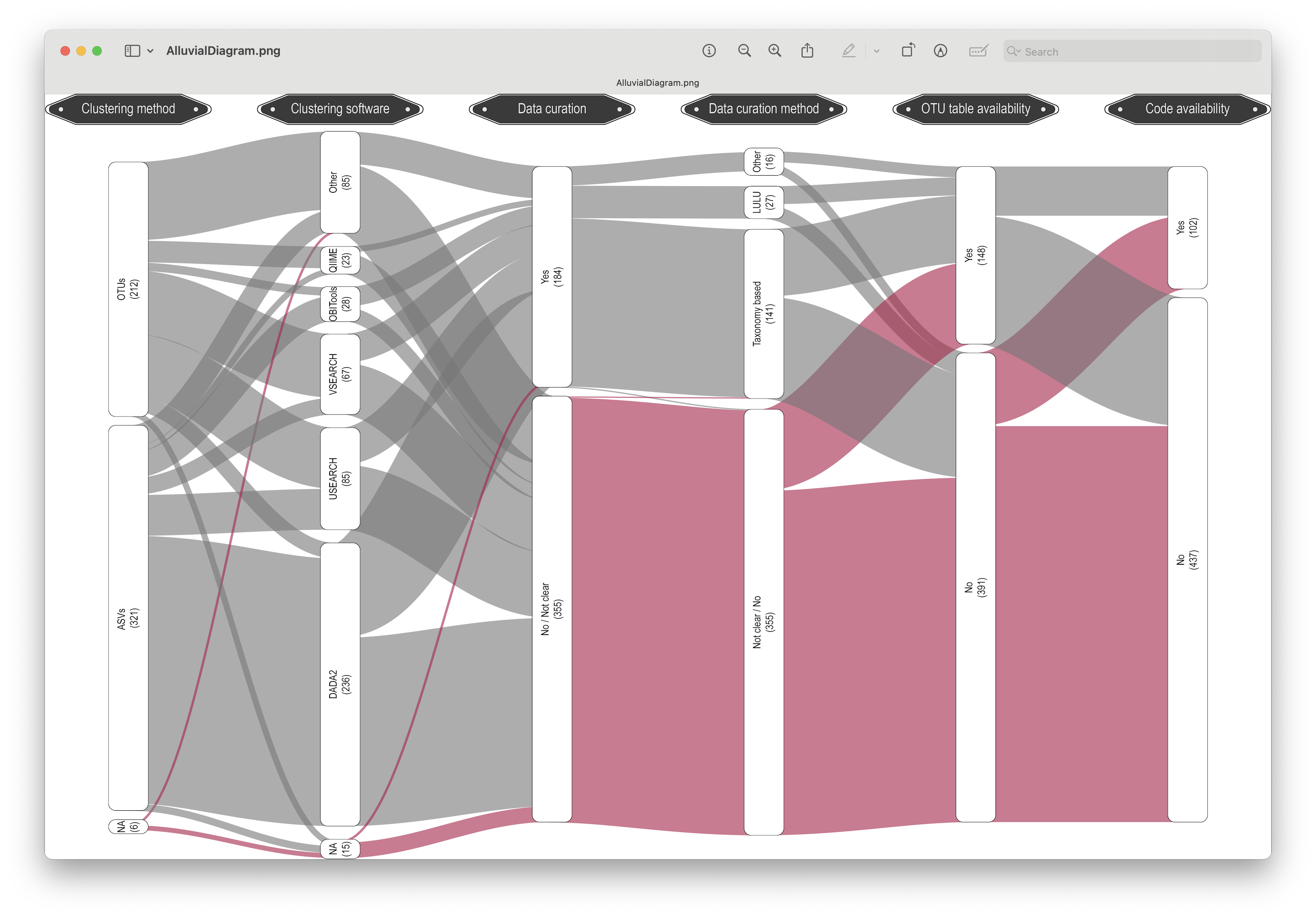
Fig. 5 : an alluvial diagram depicting the prevalence of different bioinformatic pipelines.

During this bootcamp, we will be using dada2, the most-frequently used program for the bioinformatic analysis of metabarcoding data.

4. General overview of the bioinformatic pipeline

Although software options are numerous, each pipeline follows more or less the same basic steps and accomplishes these steps using similar tools. Before we get started with coding, let’s quickly go over the main steps of the pipeline to give you a clear overview of what we will cover during this bootcamp. For each of these steps, we will provide more information when we cover those sections during the workshop.

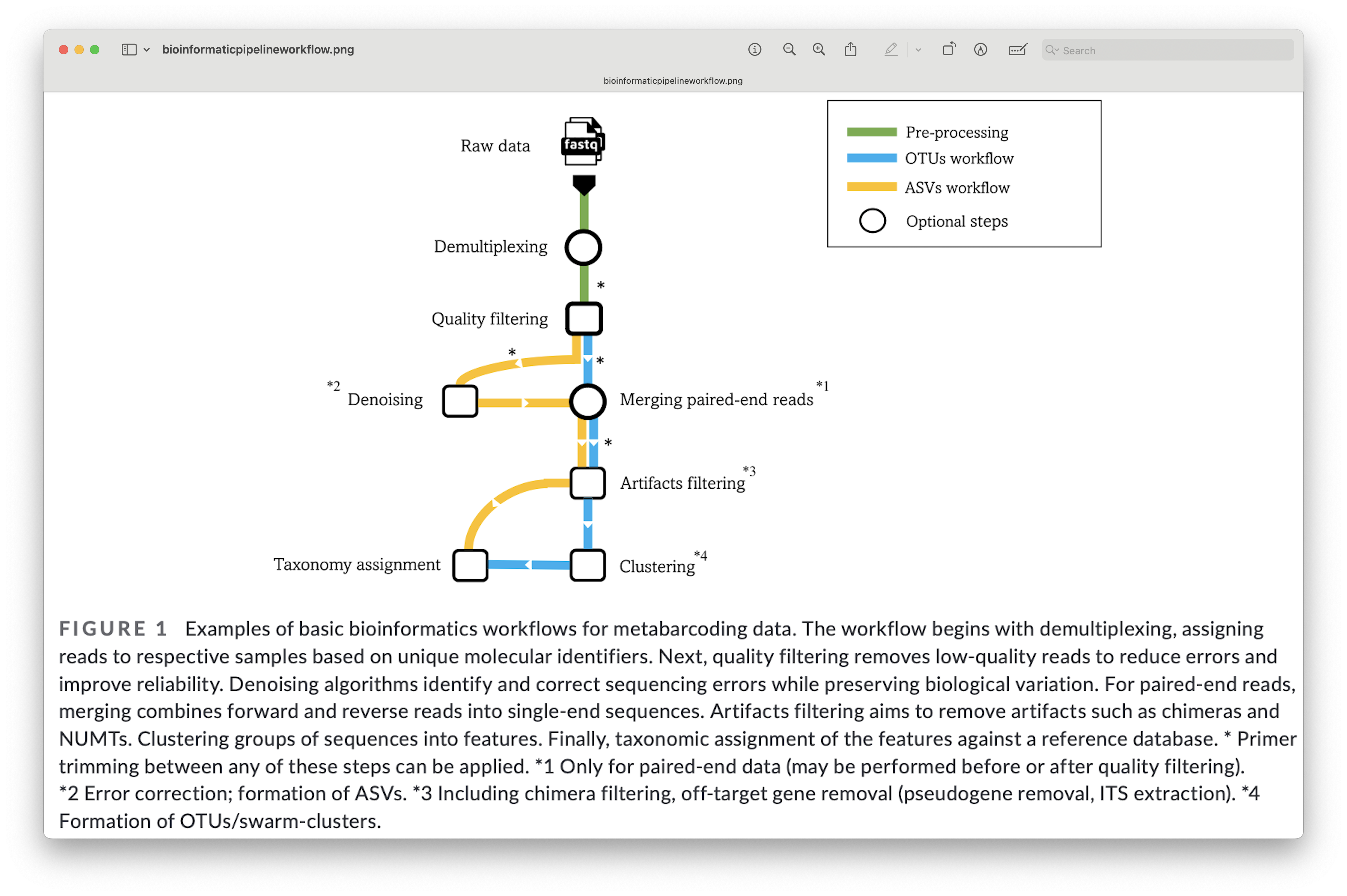
Fig. 6 : The general workflow of the bioinformatic pipeline. Copyright: Hakimzadeh et al., 2023.

5. A note on scripts and reproducible code

One final topic we need to cover before we get started with coding is the use of scripts to execute code. During this workshop, we will mainly be working in RStudio. This environment lends itself to writing code in R scripts, while still remaining interactive by enabling line-by-line code execution. While it is possible to copy-paste the provided commands/code directly in the R console or R Terminal window without using scripts, it is good practice to use scripts for the following three reasons:

1. By using scripts to execute the code, there is a written record of how the data was processed. This will make it easier for you to remember how the data was processed in the future.

2. While the sample data provided in this tutorial is small and computing steps take up a maximum of several minutes, processing large data sets can be time consuming. It is, therefore, recommended to process a small portion of the data first to test the code, modify the filenames once everything is set up, and run it on the full data set.

3. Scripts can be reused in the future by changing file names, saving you time by not having to constantly write every line of code in the Console or Terminal window. Minimising the amount needing to be written in the Console or Terminal will, also, minimise the risk of receiving error messages due to typo’s, which is the most common error message seen during bioinformatic analysis.

That is it for the intro, let’s get started with coding!