eDNA workshop HKU
Welcome to the bioinformatic and statistical analysis sessions of the eDNA workshop held at Hong Kong University!
The primary goal of the following couple of sessions are to introduce you to the analysis of eDNA metabarcoding sequence data, and ultimately make you comfortable to explore your own next-generation sequencing project. The sessions are split up into three days, with the bioinformatic analysis on the 23rd of October, taxonomy assignment on the 24th of October, and statistical analysis on the 25th of October. At the end of the three days, we hope you will be able to understand and execute the main steps in a bioinformatic pipeline, build your own custom reference database, assign a taxonomic ID to your sequences using different algorithms, and analyse metabarcoding data in a statistically correct manner.
A quick recap on last week
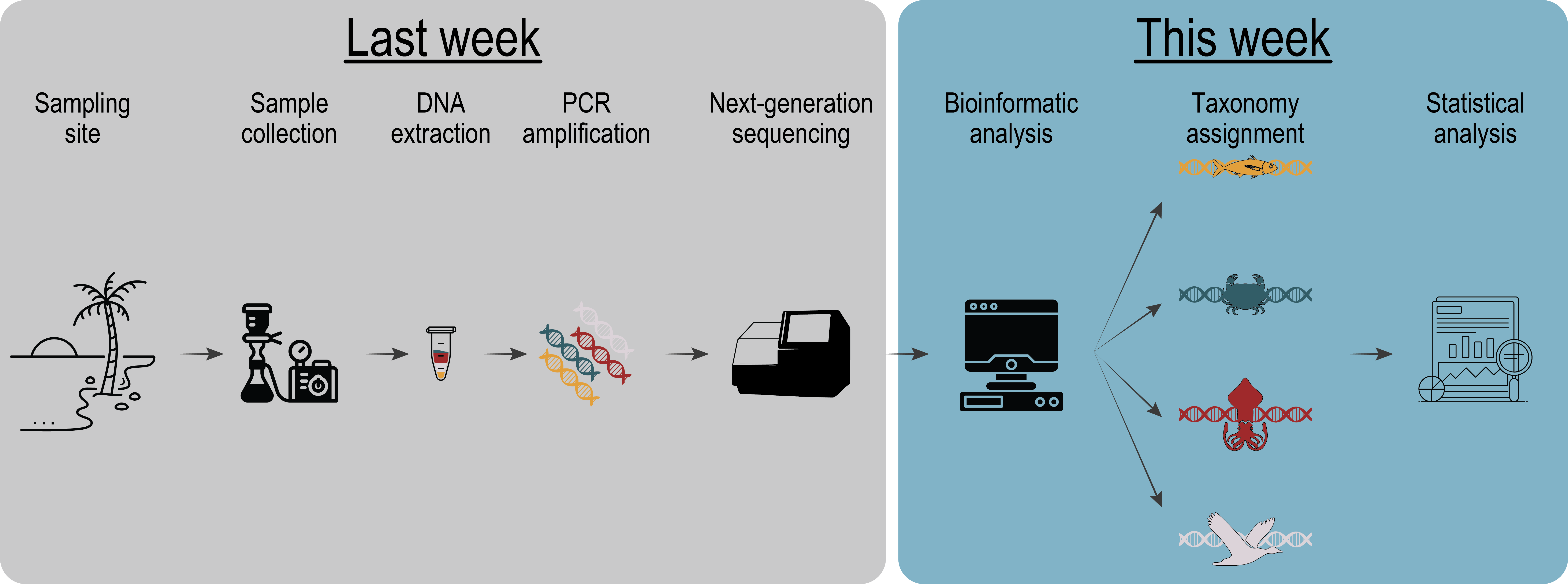
We covered a wide range of topics during the first week of this eDNA workshop, including the importance of experimental design, how to conduct field work, appropriate laboratory protocols to process low-quantity DNA samples, and various sequencing approaches.
For the following sessions, we will assume that we have submitted our library and received the sequencing data back from the sequencing service. The steps that we will cover in the next few days are:
The bioinformatic processing of the raw sequence data;
Taxonomy assignment of the biologically-relevant sequences;
The statistical analysis to answer the question of your hypothesis.

Fig. 1 : a general overview of the eDNA metabarcoding workflow from sample collection to data analysis.#
Before we get started with the bioinformatic pipeline, we will first introduce the data we will be analysing, some of the software programs available (including the ones we will use in this workshop), and the general structure of a bioinformatic pipeline to process metabarcoding data. Finally, we will go over the folder structure we suggest you use during the processing of metabarcoding data to help keep an overview of the files and ensure reproducibility of the analysis.
Experimental setup
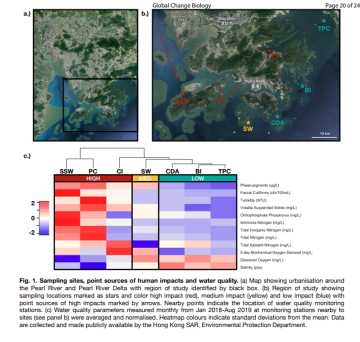
The data we will be analysing is a subset of the data from an eDNA metabarcoding experiment conducted by Dr David Baker and Dr Isis Guibert in Hong Kong, where they were interested to investigate how varying intensities of anthropogenic impacts alter the biodiversity in the Pearl River Delta. To test this, they deployed 3 ARMS (Autonomous Reef Monitoring Structures) at each site over summer, including two highly impacted (SSW: San Shek Wan; PC: Peng Chau) and two sites with low human impact (BI: Bluff Island; TPC: Tung Ping Chau). After deployment, the ARMS structure was taken apart by detaching the individual plates. Motile organisms were removed first by hand and then through sieves in two size fractions, including 100 µm and 500 µm. The plate surfaces were then photographed and sessile organisms were scraped off each plate and homogenized in a blender. DNA metabarcoding using a ~313 bp fragment of the cytochrome c oxidase subunit I (Leray & Knowlton, 2015) was conducted to asses bulk diversity between the highly impacted and low impact sites. Size fractions were sequenced separately, allowing us to investigate diversity differences within each size fraction, as well as the combined diversity. During the bioinformatic and statistical analysis, we will be processing the 100 µm and 500 µm size fractions from the two highly-impacted and two low-impacted locations.

Fig. 2 : The experimental design of the data we will be analysing during the next few days. Note that this is the information of the full experiment. Please read the section above to provide an overview of what subset will be analysed during this workshop.#
A note on software programs
The popularity of metabarcoding research, both in the bacterial and eukaryote kingdom, has resulted in the development of a myriad of software packages and pipelines. Furthermore, software packages are continuously updated with new features, as well as novel software programs being designed and published. We will be using several software programs and R packages during this workshop. However, we would like to stress that the pipeline used in the workshop is by no means better than other pipelines and we urge you to explore alternative software programs and trial them with your own data after this workshop.
Metabarcoding software programs can generally be split up into two categories, including:
stand-alone programs that are self-contained: These programs usually incorporate novel functions or alterations on already-existing functions. Programs can be developed for a specific task within the bioinformatic pipeline or can execute multiple or all steps in the bioinformatic pipeline. Examples of such programs are: Mothur, USEARCH, VSEARCH, cutadapt, dada2, OBITools3.
wrappers around existing software: These programs attempt to provide an ecosystem for the user to complete all steps within the bioinformatic pipeline without needing to reformat documents or change the coding language. Examples of such programs are: QIIME2 and JAMP.
The list of software programs and R packages we will be using during this tutorial:
Bioinformatic processing (Terminal):
Taxonomy assignment (Terminal):
CRABS: build custom curated reference databases.
SINTAX: k-mer based classifier to assign a taxonomic ID to sequences.
IDTAXA (RStudio): machine learning classifier to assign a taxonomic ID to sequences.
BLAST: local alignment classifier to assign a taxonomic ID to sequences.
Statistical analysis (RStudio):
Phyloseq: R package to explore metabarcoding data.
iNEXT.3D: R package to calculate inter- and extrapolation of alpha diversity measures.
ape: R package to build multiple sequence alignments and phylogenetic trees.
microbiome: R package as an extension to phyloseq.
indicspecies: R package to calculate indicator species values
vegan: R package to calculate various alpha and beta diversity measures.
ggtree: build phylogenetic tree graphics.
Warning
Some software programs change the standard structure of your file to be compatible with the functions implemented within the program. When implementing several software programs in your bioinformatic pipeline, such modifications in the file structure could lead to incompatability issues when switching to the next program in your pipeline. It is, therefore, important to understand how a specific program changes the structure of the sequence file and learn how these modifications can be reverted back (through simple python, bash, or R scripts). We will talk a little bit more about file structure and conversion throughout the workshop.
General overview of the bioinformatic pipeline
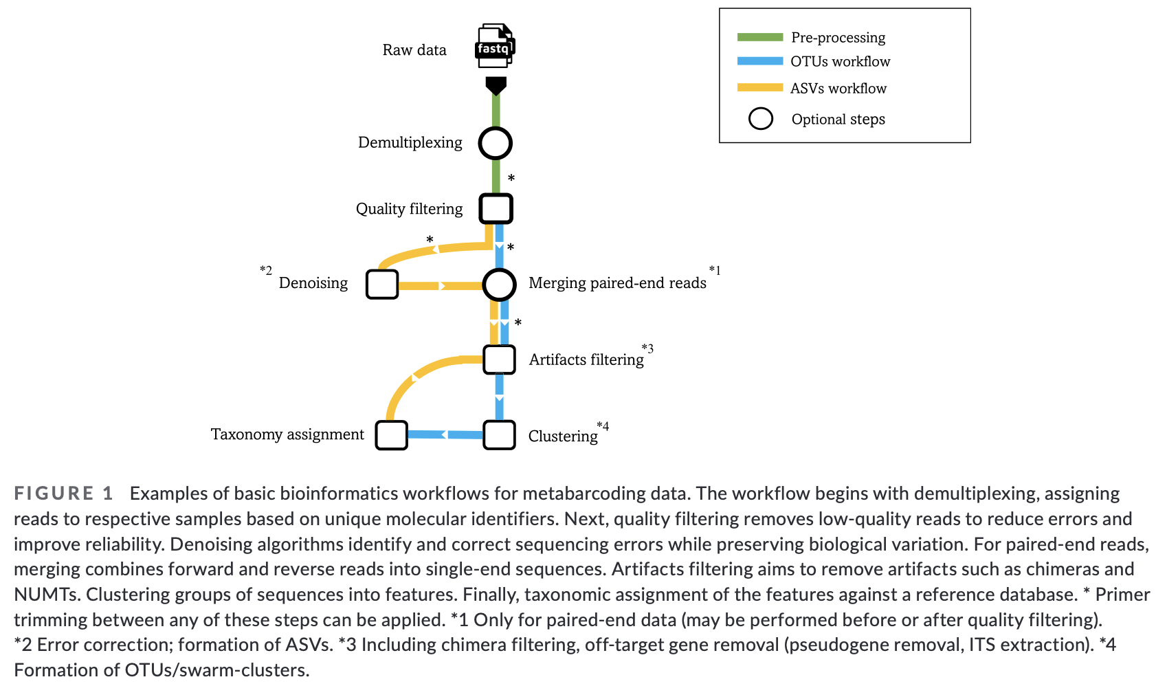
Although software options are numerous, each pipeline follows more or less the same basic steps and accomplishes these steps using similar tools. Before we get started with coding, let’s quickly go over the main steps of the pipeline to give you a clear overview of what we will cover today. For each of these steps, we will provide more information when we cover those sections during the workshop.

Fig. 3 : The general workflow of the bioinformatic pipeline. Copyright: Hakimzadeh et al., 2023.#
A note on scripts and reproducible code
One final topic we need to cover before we get started with coding is the use of scripts to execute code. During this workshop, we will create very small and simple scripts that contain the code used to process the sequencing data. While it is possible to run the commands directly in the Terminal window without using scripts, it is good practice to use this method for the following three reasons:
By using scripts to execute the code, there is a written record of how the data was processed. This will make it easier for you to remember how the data was processed in the future.
While the sample data provided in this tutorial is small and computing steps take up a maximum of several minutes, processing large data sets can be time consuming. It is, therefore, recommended to process a small portion of the data first to test the code, modify the filenames once everything is set up, and run it on the full data set.
Scripts can be reused in the future by changing file names, saving you time by not having to constantly write every line of code in the terminal. Minimising the amount needing to be written in the terminal will, also, minimise the risk of receiving error messages due to typo’s.
