Statistical analysis#
1. Introduction#
During this section, we will cover some common statistical analyses that are conducted in eDNA metabarcoding research. Such methods mainly focus on alpha and beta diversity comparisons between sites/treatments.
Important
Before we start with the statistical analysis, it is essential to keep an overview of the experimental design. Basically, we want to determine if we can observe differences in the biological community between sites that are highly impacted by anthropogenic stressors and sites that are less impacted by anthropogenic stressors. To test this, 3 ARMS (Autonomous Reef Monitoring Structures) were placed at each site, including 2 sites identified as highly impacted and two sites identified with low impact. After deployment, the biological community was subsetted by size, including 100 µm and 500 µm.
All of this means that we have 2 DNA samples per ARMS, 3 ARMS per site, and 4 sites = 24 samples.
For the statistical comparison, we could test differences between high and low impacted sites for each size fraction of the biological community separately, as well as a combined approach of both size fractions. During this tutorial, we will only cover the analysis of the separate size fractions to keep things simple.
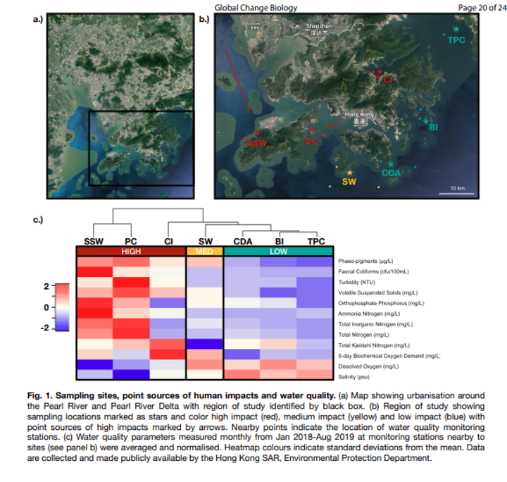
Fig. 51 : The experimental design of the data we will be analysing during the next few days. Note that this is the information of the full experiment. Please read the section above to provide an overview of what subset will be analysed during this workshop.#
2. Reading/Parsing data#
Similarly to the previous section, most code will be run in R, unless specified otherwise. Therefore, let us open a new R script and save it as sequenceData/1-scripts/statisticalAnalysis.R. We can copy-paste the R code below into this script to run all the code. We can set up the R environment by specifying the working directory and loading all the necessary libraries.
#########################
# PREPARE R ENVIRONMENT #
#########################
library(Biostrings)
library(phyloseq)
library(ggplot2)
library(vegan)
library(iNEXT.3D)
library(microbiome)
library(ape)
library(scales)
library(readxl)
library(tidyverse)
library(ampvis2)
library(car)
library(FSA)
library(dplyr)
library(agricolae)
library(speedyseq)
library(BiodiversityR)
library(indicspecies)

# set working directory
setwd('/Users/gjeunen/Documents/work/lectures/HKU2023/tutorial/sequenceData/8-final')
We begin by reading the files into R, including the filtered frequency table sequenceData/8-fianl/zotutableFiltered.txt, the updated metadata file sequenceData/0-metadata/sampleMetadataFiltered.txt, the filtered ZOTU sequence file sequenceData/8-final/zotusFiltered.fasta, and the updated taxonomy table sequenceData/8-final/taxonomyFiltered.txt.
##################
# READ DATA IN R #
##################
metaData <- read.table('../0-metadata/sampleMetadataFiltered.txt', header = TRUE, sep = '\t', row.names = 1, check.names = FALSE, comment.char = '')
freqTable <- read.table('zotutableFiltered.txt', header = TRUE, sep = '\t', row.names = 1, check.names = FALSE, comment.char = '')
taxonomyTable <- read.table('taxonomyFiltered.txt', header = TRUE, sep = '\t', row.names = 1, check.names = FALSE, comment.char = '')
sequenceTable <- readDNAStringSet('zotusFiltered.fasta')
Once the data is read into R, we can import the dataframes into phyloseq as a single phyloseq object.
# 1. import dataframes into phyloseq
OTU = otu_table(freqTable, taxa_are_rows = TRUE)
TAX = tax_table(as.matrix(taxonomyTable))
META = sample_data(metaData)
physeq = merge_phyloseq(OTU, TAX, META, sequenceTable)
physeq
Output
> physeq
phyloseq-class experiment-level object
otu_table()   OTU Table:         [ 865 taxa and 24 samples ]
sample_data() Sample Data:       [ 24 samples by 32 sample variables ]
tax_table()   Taxonomy Table:    [ 865 taxa by 9 taxonomic ranks ]
refseq()      DNAStringSet:      [ 865 reference sequences ]
3. Summary stats#
One of the first things we will look at are some summary statistics on read number prior and post quality filtering, as well as average read number per sample, number of taxa, most abundant and most frequently detected taxa, read count in negative controls, taxa observed in negative controls, sample drop out, etc. These numbers are usually reported in the first paragraph of the results section in eDNA metabarcoding publications.
Most of these numbers have already been reported on during the bioinformatic and data processing session. For example, we know that after the bioinformatic processing of the raw sequencing data, we ended up with 2,195,816 reads across 1,345 ZOTU sequences. Additionally, we know that during data pre-processing, we filtered the total number of ZOTU sequences to 865 and after contaminant and abundance filtering, we ended up with a total of 1,768,932 reads.
Information about the negative controls has also been provided during the data pre-processing session. For example, we know that there were 99 ZOTUs with a positive detection in the negative controls, including the top 9 most-abundant ZOTU sequences in our data set. Of those 99 ZOTUs with a positive detection in the negative controls, total read count reached 287 (0.01%) and most abundant read count for a single detection in the negative controls was 12 reads and 23 when summed across all negative control samples. This highest number of reads was observed for ZOTU 1, which is assigned to the class Hexanauplia.
Another aspect that is frequently mentioned is information about the taxonomic assignment. For the tutorial data, 58 ZOTUs did not achieve a taxonomic ID through BLAST (the taxonomic ID we used during the data pre-processing steps). Removal of these signals resulted in a reduction of 14,735 reads from the final data set.
Important
During the tutorial, we have not gone over the quality of the taxonomic assignment. Some studies will filter out sequences with low-quality taxonomic ID scores or set arbitrary thresholds at which level the taxonomic ID should be set. Please keep in mind that this is something you can and should do for your data set as well if you would like to focus on a taxonomic-dependent analysis.
Finally, we can report that we used the LULU algorithm to identify artefact sequences. Through this approach, 369 child or artefact sequences were merged with their parent.
To get some further summary statistics on the final frequency table (such as minimum and maximum read count, average read count, ZOTUs summing to 0, etc.) we can make use of multiple functions within the phyloseq and microbiome R packages.
#################
# SUMMARY STATS #
#################
summarize_phyloseq(physeq)
summary(readcount(physeq))
sd(readcount(physeq))
se <- function(x) sd(x)/sqrt(length(x))
se(readcount(physeq))
Output
[[1]]
[1] "1] Min. number of reads = 35142"

[[2]]
[1] "2] Max. number of reads = 126301"

[[3]]
[1] "3] Total number of reads = 1768932"

[[4]]
[1] "4] Average number of reads = 73705.5"

[[5]]
[1] "5] Median number of reads = 69433.5"

[[6]]
[1] "7] Sparsity = 0.785452793834297"

[[7]]
[1] "6] Any OTU sum to 1 or less? NO"

[[8]]
[1] "8] Number of singletons = 0"

[[9]]
[1] "9] Percent of OTUs that are singletons \n        (i.e. exactly one read detected across all samples)0"

[[10]]
[1] "10] Number of sample variables are: 32"

[[11]]
 [1] "sample_name"                     "ARMS_ID"
 [3] "SAMPLE"                          "sampleSite"
 [5] "TargetLoci"                      "impact"
 [7] "replicateLabel"                  "island"
 [9] "siteDetails"                     "StationID"
[11] "habitat"                         "PercentCoralCover"
[13] "locality"                        "decimalLongitude"
[15] "decimalLatitude"                 "actualDeploymentDate"
[17] "actualRecoveryDate"              "totalmonth"
[19] "Month_Ret"                       "Ret_ID"
[21] "Temperature...C."                "Salinity..psu."
[23] "Dissolved.Oxygen..mg.L."         "Turbidity..NTU."
[25] "Total.Inorganic.Nitrogen..mg.L." "Total.Nitrogen..mg.L."
[27] "Chlorophyll.a..μg.L."            "Faecal.Coliforms..cfu.100mL."
[29] "station.gov"                     "EPD_date_from"
[31] "EPD_date_to"                     "comments"
Output
> summary(readcount(physeq))
   Min. 1st Qu.  Median    Mean 3rd Qu.    Max.
  35142   54186   69434   73706   89468  126301

> sd(readcount(physeq))
[1] 24364.47

> se <- function(x) sd(x)/sqrt(length(x))
> se(readcount(physeq))
[1] 4973.378
Besides read count per sample, we can also investigate the most abundant (with regards to read count) and most frequently detected (occurrence count) taxa through some simple for loops in R.
# 1. list 10 most abundant (read count) taxa
for (x in top_taxa(physeq, n = 10)) {
  taxa <- tax_table(physeq)[x, ]
  count <- sum(otu_table(physeq)[x, ])
  print(taxa)
  print(count)
  print(count/sum(otu_table(physeq))*100)
}

# 1. list 10 most frequently detected (occurrences) taxa
for (x in top_taxa(microbiome::transform(physeq, 'pa'), n = 10)) {
  taxa <- tax_table(physeq)[x, ]
  count <- sum(otu_table(microbiome::transform(physeq, 'pa'))[x, ])
  print(taxa)
  print(count)
  print(count/ncol(freqTable)*100)
}
Output
Taxonomy Table:     [1 taxa by 9 taxonomic ranks]:
       kingdom     phylum       class         order        family       genus            species          pident    qcov
zotu.1 "Eukaryota" "Arthropoda" "Hexanauplia" "Cyclopoida" "Cyclopidae" "Cyclopidae_nan" "Cyclopidae_sp." " 75.421" " 95"
[1] 222411
[1] 12.57318
Taxonomy Table:     [1 taxa by 9 taxonomic ranks]:
       kingdom     phylum       class       order       family           genus       species                 pident    qcov
zotu.2 "Eukaryota" "Arthropoda" "Arachnida" "Opiliones" "Nemastomatidae" "Mitostoma" "Mitostoma_chrysomelas" " 76.596" " 89"
[1] 168289
[1] 9.513594
Taxonomy Table:     [1 taxa by 9 taxonomic ranks]:
       kingdom     phylum       class          order      family      genus     species  pident    qcov
zotu.3 "Eukaryota" "Arthropoda" "Malacostraca" "Decapoda" "Alpheidae" "Athanas" "parvus" " 99.681" "100"
[1] 137326
[1] 7.763215
Taxonomy Table:     [1 taxa by 9 taxonomic ranks]:
       kingdom     phylum     class        order          family       genus         species                 pident    qcov
zotu.7 "Eukaryota" "Annelida" "Polychaeta" "Phyllodocida" "Nereididae" "Platynereis" "Platynereis_dumerilii" " 84.158" " 96"
[1] 65860
[1] 3.72315
Taxonomy Table:     [1 taxa by 9 taxonomic ranks]:
       kingdom     phylum     class        order          family       genus         species pident    qcov
zotu.8 "Eukaryota" "Annelida" "Polychaeta" "Phyllodocida" "Nereididae" "Platynereis" "HK01"  "100.000" "100"
[1] 57249
[1] 3.23636
Taxonomy Table:     [1 taxa by 9 taxonomic ranks]:
        kingdom     phylum       class          order      family             genus            species  pident    qcov
zotu.10 "Eukaryota" "Arthropoda" "Malacostraca" "Decapoda" "Rhynchocinetidae" "Rhynchocinetes" "brucei" "100.000" "100"
[1] 47045
[1] 2.659514
Taxonomy Table:     [1 taxa by 9 taxonomic ranks]:
        kingdom     phylum       class          order      family       genus            species pident    qcov
zotu.11 "Eukaryota" "Arthropoda" "Malacostraca" "Decapoda" "Pilumnidae" "Pilumnidae_nan" "HK03"  " 79.769" " 55"
[1] 45386
[1] 2.565729
Taxonomy Table:     [1 taxa by 9 taxonomic ranks]:
       kingdom     phylum     class        order          family       genus         species pident    qcov
zotu.9 "Eukaryota" "Annelida" "Polychaeta" "Phyllodocida" "Nereididae" "Platynereis" "HK01"  "100.000" "100"
[1] 45334
[1] 2.562789
Taxonomy Table:     [1 taxa by 9 taxonomic ranks]:
        kingdom     phylum     class         order         family     genus         species                    pident    qcov
zotu.16 "Eukaryota" "Chordata" "Actinopteri" "Gobiiformes" "Gobiidae" "Tridentiger" "Tridentiger_nudicervicus" "100.000" " 97"
[1] 32197
[1] 1.820138
Taxonomy Table:     [1 taxa by 9 taxonomic ranks]:
        kingdom     phylum       class     order     family     genus     species             pident    qcov
zotu.13 "Eukaryota" "Arthropoda" "Insecta" "Diptera" "Muscidae" "Muscina" "Muscina_pascuorum" " 80.412" " 93"
[1] 30681
[1] 1.734436
Output
Taxonomy Table:     [1 taxa by 9 taxonomic ranks]:
        kingdom     phylum     class        order      family      genus          species               pident    qcov
zotu.57 "Eukaryota" "Annelida" "Polychaeta" "Spionida" "Spionidae" "Boccardiella" "Boccardiella_hamata" " 85.761" " 99"
[1] 24
[1] 100
Taxonomy Table:     [1 taxa by 9 taxonomic ranks]:
         kingdom     phylum     class        order      family      genus          species               pident    qcov
zotu.122 "Eukaryota" "Annelida" "Polychaeta" "Spionida" "Spionidae" "Boccardiella" "Boccardiella_hamata" " 84.091" " 98"
[1] 23
[1] 95.83333
Taxonomy Table:     [1 taxa by 9 taxonomic ranks]:
        kingdom     phylum       class          order      family      genus       species pident    qcov
zotu.14 "Eukaryota" "Arthropoda" "Malacostraca" "Decapoda" "Xanthidae" "Leptodius" "HK01"  "100.000" "100"
[1] 19
[1] 79.16667
Taxonomy Table:     [1 taxa by 9 taxonomic ranks]:
         kingdom     phylum       class         order          family      genus     species            pident    qcov
zotu.155 "Eukaryota" "Arthropoda" "Thecostraca" "Balanomorpha" "Balanidae" "Balanus" "Balanus_trigonus" "100.000" "100"
[1] 19
[1] 79.16667
Taxonomy Table:     [1 taxa by 9 taxonomic ranks]:
       kingdom     phylum     class        order          family       genus         species pident    qcov
zotu.8 "Eukaryota" "Annelida" "Polychaeta" "Phyllodocida" "Nereididae" "Platynereis" "HK01"  "100.000" "100"
[1] 19
[1] 79.16667
Taxonomy Table:     [1 taxa by 9 taxonomic ranks]:
        kingdom     phylum       class       order         family          genus       species              pident    qcov
zotu.21 "Eukaryota" "Arthropoda" "Diplopoda" "Polydesmida" "Xystodesmidae" "Brachoria" "Brachoria_laminata" " 76.654" " 81"
[1] 18
[1] 75
Taxonomy Table:     [1 taxa by 9 taxonomic ranks]:
        kingdom     phylum     class        order          family       genus      species        pident    qcov
zotu.79 "Eukaryota" "Annelida" "Polychaeta" "Phyllodocida" "Hesionidae" "Syllidia" "Syllidia_sp." "100.000" "100"
[1] 18
[1] 75
Taxonomy Table:     [1 taxa by 9 taxonomic ranks]:
         kingdom     phylum       class         order          family      genus     species            pident    qcov
zotu.221 "Eukaryota" "Arthropoda" "Thecostraca" "Balanomorpha" "Balanidae" "Balanus" "Balanus_trigonus" " 99.681" "100"
[1] 17
[1] 70.83333
Taxonomy Table:     [1 taxa by 9 taxonomic ranks]:
         kingdom     phylum     class        order      family      genus      species             pident    qcov
zotu.388 "Eukaryota" "Annelida" "Polychaeta" "Spionida" "Spionidae" "Polydora" "Polydora_haswelli" " 97.444" "100"
[1] 17
[1] 70.83333
Taxonomy Table:     [1 taxa by 9 taxonomic ranks]:
        kingdom     phylum       class         order          family      genus          species                    pident    qcov
zotu.52 "Eukaryota" "Arthropoda" "Thecostraca" "Balanomorpha" "Balanidae" "Amphibalanus" "Amphibalanus_reticulatus" "100.000" "100"
[1] 17
[1] 70.83333
4. Data exploration#
We already covered several data exploration techniques in the previous sections. For example, we created a phylogenetic tree to investigate differences in detection frequency of Cnidarian ZOTUs between low and high impact sites in the Phylogenetic tree section. Additionally, we investigated if sufficient sequencing depth was achieved for samples through rarefaction curves in the Data pre-processing section.
4.1 Phyloseq functions#
The phyloseq R package itself also provides some basic graphs to explore your metabarcoding data even further, including bar graphs (plot_bar), heat maps (plot_heatmap), richness (plot_richness), basic tree figures (plot_tree), and ordination graphs (plot_ordination; more on this in section 6. Beta diversity). Below are some examples of these plotting functions. Note that you can expand on this by subsetting the data in a meaningful manner. More information about the phyloseq R package and some excellent tutorials can be found on the phyloseq webpage.
4.1.1 Bar plots#
# 1. create bar plot of samples coloured by phylum, 2. group by impact, 3. facet by location, 4. use ggplot to remove ZOTU lines
plot_bar(physeq, fill = "phylum")
plot_bar(physeq, x = 'impact', fill = 'phylum')
plot_bar(physeq, x = 'SAMPLE', fill = 'phylum', facet_grid=~impact)
p <- plot_bar(physeq, x = 'SAMPLE', fill = 'phylum', facet_grid=~impact)
p + geom_bar(aes(color=phylum, fill=phylum), stat="identity", position="stack")
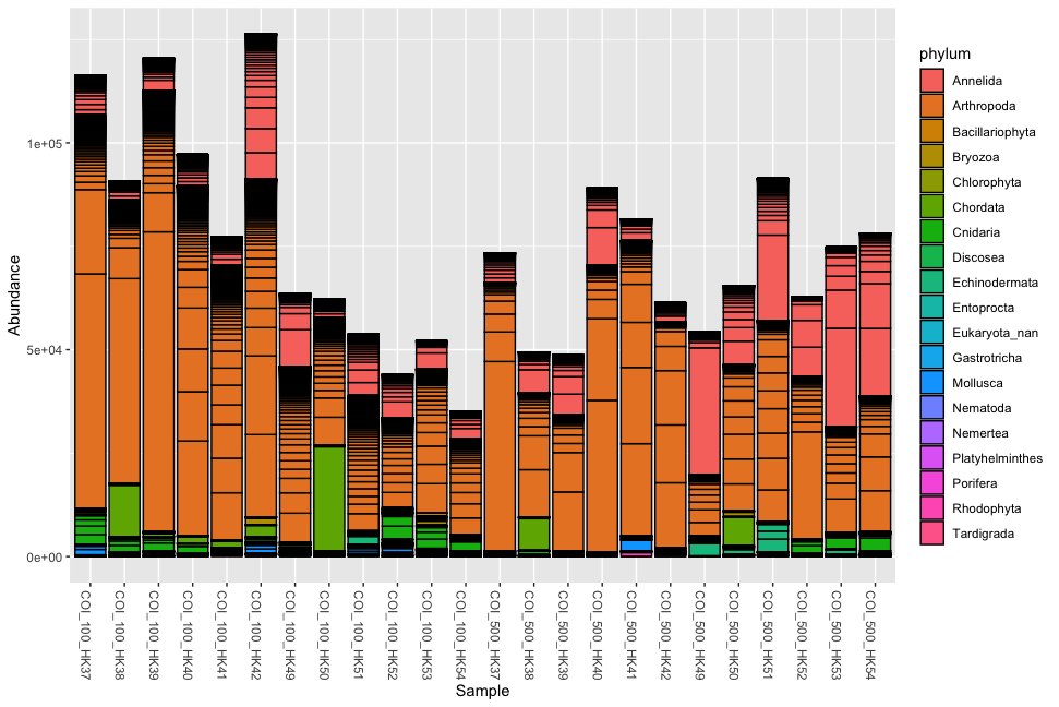
Fig. 52 : Simple phyloseq bar plot of samples whereby abundance of ZOTU sequences are coloured by phylum ID.#
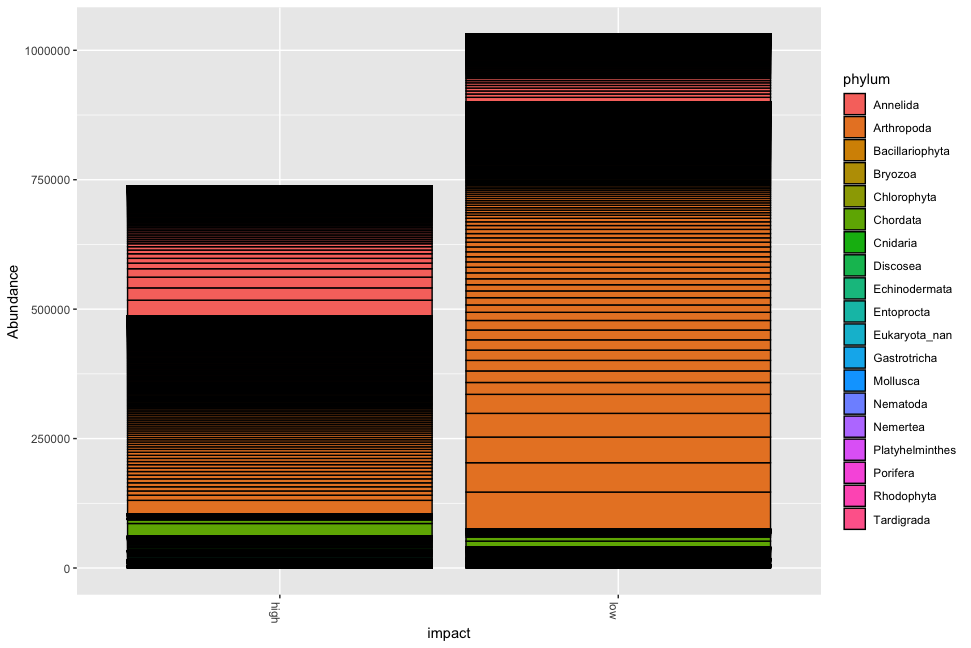
Fig. 53 : Simple phyloseq bar plot of samples whereby abundance of ZOTU sequences are coloured by phylum ID and samples are merged based on impact metadata information.#
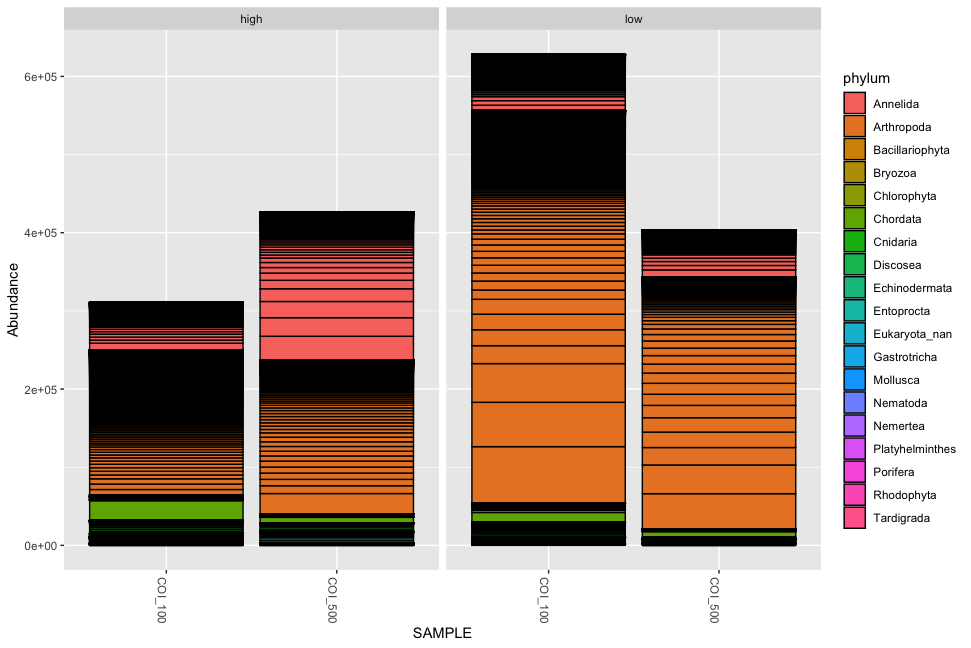
Fig. 54 : Simple phyloseq bar plot of samples whereby abundance of ZOTU sequences are coloured by phylum ID, samples are merged based on size fraction and facetted by impact metadata information.#
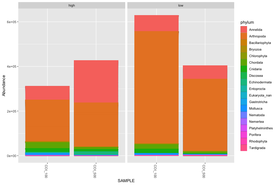
Fig. 55 : Simple phyloseq bar plot as above, but whereby ggplot is used to remove the black ZOTU lines.#
4.1.2 Heat maps#
# 1. plot simple heatmap, 2. plot heatmap with relabeled x-axis labels and different colours
plot_heatmap(physeq)
plot_heatmap(physeq, sample.label = 'sampleSite', low = '#66CCFF', high = '#000033', na.value = 'white')
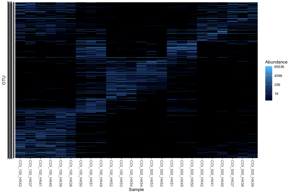
Fig. 56 : Simple phyloseq heat map.#
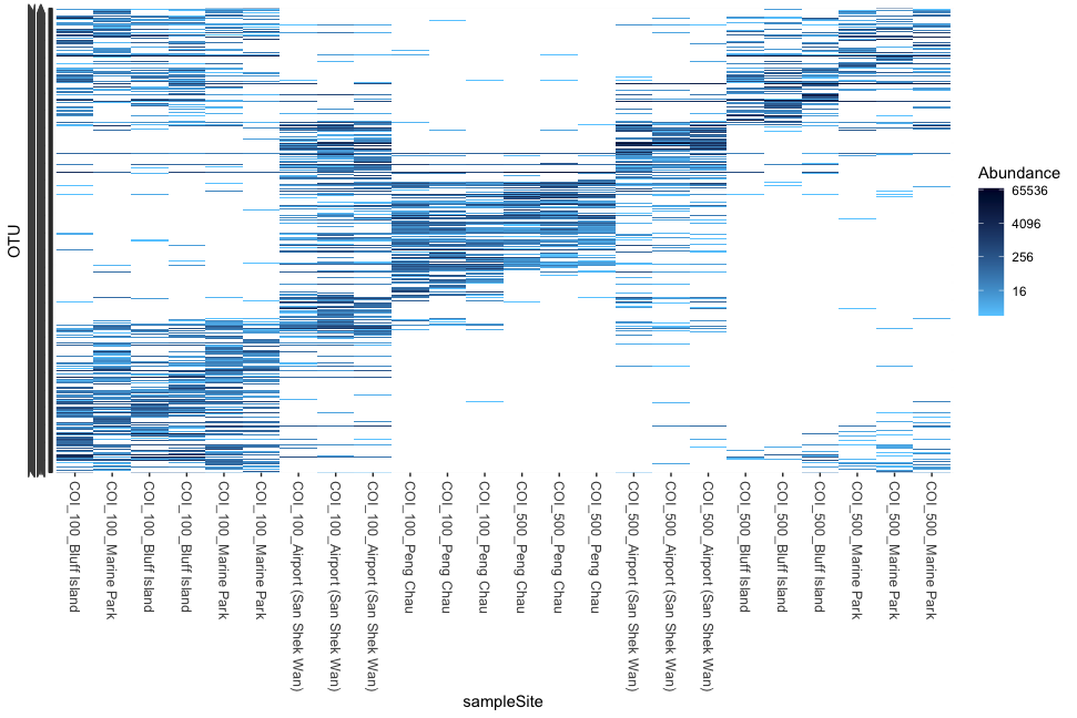
Fig. 57 : Simple phyloseq heat map whereby x-axis labels are altered and heat map colours are changed.#
4.1.3 Richness#
# 1. plot richness
plot_richness(physeq, x="impact", color="SAMPLE", measures = c('Observed', 'Chao1', 'Shannon', 'Simpson'))
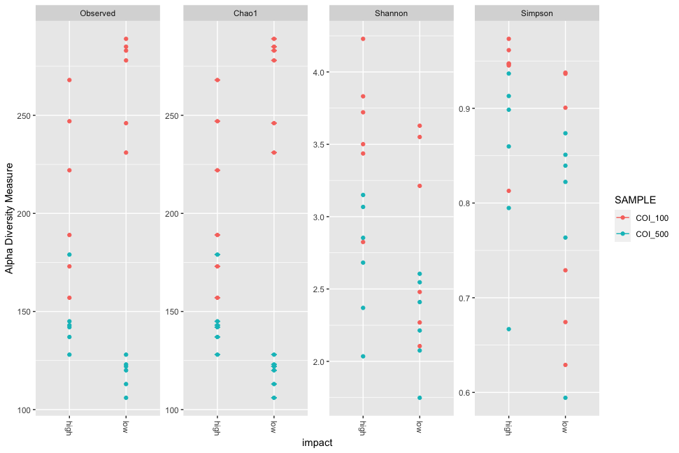
Fig. 58 : Simple phyloseq multiple richness measurements grouped by low and high impact and coloured by size fraction.#
5. Alpha diversity#
In short, alpha diversity is the characterisation of diversity within a site. Researchers use this characterisation to quantify how diverse different systems are. Over the last century, a myriad of approaches and tools have been developed to perform such operations, each embedded within a statistical background. One important aspect, and where these various approaches can differ, is the differential weighing of abundant and rare species. The simplest approach, and most-frequently used in metabarcoding research, is species richness, which only considers the presence or absence of a species. However, OTUs in a system are rarely distributed evenly; thus using richness is rarely the best approach with which to reflect the diversity of a system. Other popular approaches that do account for the evenness of a system are the Shannon index and the Simpson index. However, it is important to note that both are not acutal measures of diversity. Shannon measures entropy and therefore yields the uncertainty in species identity of a randomly chosen species in the system, while Simpson provides the probability that two randomly chosen species actually belong to different species. Hence, both Shannon and Simpson are difficult to interpret and are not intuitive. For example, a doubling of the species in a system (10 compared to 20 species for example), does not yield double the value of Shannon or Simpson. Fortunately, these indices belong to a single statistical framework. Hence, we can rework these formulas and calculate the actual diversities using so-called Hill numbers (qD), which is a simple statistical framework allowing us to calculate various diversity metrics using a single system. Within the Hill number framework, q = 0 represents species richness, q = 1 represents the exponential of the Shannon index, and q = 2 represents the inverse of the Simpson index. For more information, we can have a look at the figure below. I also strongly suggest reading the excellent paper by Alberdi & Gilbert, 2019, which covers all of this in much more detail and in context of a metabarcoding approach. They also provide all the essential citations of the original statistical framework development.
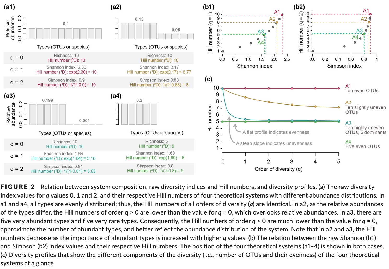
Fig. 59 : Introduction to the Hill number statistical framework. Copyright: Alberdi & Gilbert, 2019.#
For the alpha diversity analysis in this tutorial, we will be using the Hill number framework. However, since metabarcoding approaches do not hold true abundance information, or at least the correlation between eDNA signal strength and species abundance is very weak, we will need to approximate relative abundance measurements from our data set. We can do so by using a so-called incidence-based approach. This approach works by transforming the data set to presence-absence and combining multiple samples from the same site/treatment to obtain the relative abundance information.
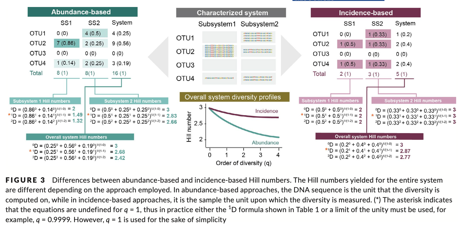
Fig. 60 : Introduction to incidence-based data transformation. Copyright: Alberdi & Gilbert, 2019.#
5.1 Species accumulation curves#
To expand upon rarefaction curves, whereby the plateauing of the curves indicate sufficient sequencing coverage was achieved for samples, we can take advantage of the fact that we have multiple ARMS (3) at each site. Transforming our frequency table to presence-absence data allows us to transform our data set to an incidence-raw format. When merging samples based on site location, we can form an incidence-frequency table to approximate a semi-quantitative data set. Through inter- and extrapolation calculations, we can draw and investigate alpha diversity accumulation curves (similar to species accumulation curves). Such an approach is implemented in the iNEXT.3D R package. These graphs will help us determine if sufficient sampling was conducted at each site, based on the plateauing of the curves, similar to the rarefaction curves we discussed in section Data pre-processing. Unlike the rarefaction curves we generated earlier, iNEXT.3D can extrapolate alpha diversity numbers beyond the number of samples collected. By default, the extrapolation value is set to double the number of samples. We will leave this default value (in our case 6 samples; double of the 3 ARMS per site), as increasing this value increases the error profile. We can also specify the different Hill number we want to investigate through the q parameter.
First, we need to subset our phyloseq object into two different objects, one containing the information about the 100 µm size fraction and one containing the information about the 500 µm size fraction.
############
# iNEXT.3D #
############
# 1. subset data based on size fractions
physeq.100 = subset_samples(physeq, SAMPLE == "COI_100")
physeq.500 = subset_samples(physeq, SAMPLE == "COI_500")
Next, we need to convert our data format to the iNEXT.3D specific format of incidence-frequency. We can use the code below to achieve this reformatting of the dataframe. We need to run this twice, once for each subsetted dataframe.
# 1. reformat data to iNEXT.3D standard for 100 size fraction
categories.100 <- unique(sample_data(physeq.100)$sampleSite)
split_physeq_list_100 <- list()
for (category in categories.100) {
  sub_physeq.100 <- subset_samples(microbiome::transform(physeq.100, 'pa'), sampleSite == category)
  split_physeq_list_100[[category]] <- otu_table(sub_physeq.100)
}
matrix_list.100 <- lapply(split_physeq_list_100, function(x) {
  otu_table <- as(x, "matrix")
  return(otu_table)
})
# Create a list named "data" to store matrices
matrix_list.100 <- list(data = list())
# Convert each split phyloseq object into a matrix and store it under "data"
for (category in categories.100) {
  otu_table <- as(otu_table(split_physeq_list_100[[category]]), "matrix")
  matrix_list.100[["data"]][[category]] <- otu_table
}

# 1. reformat data to iNEXT.3D standard for 500 size fraction
categories.500 <- unique(sample_data(physeq.500)$sampleSite)
split_physeq_list_500 <- list()
for (category in categories.500) {
  sub_physeq.500 <- subset_samples(microbiome::transform(physeq.500, 'pa'), sampleSite == category)
  split_physeq_list_500[[category]] <- otu_table(sub_physeq.500)
}
matrix_list.500 <- lapply(split_physeq_list_500, function(x) {
  otu_table <- as(x, "matrix")
  return(otu_table)
})
# Create a list named "data" to store matrices
matrix_list.500 <- list(data = list())
# Convert each split phyloseq object into a matrix and store it under "data"
for (category in categories.500) {
  otu_table <- as(otu_table(split_physeq_list_500[[category]]), "matrix")
  matrix_list.500[["data"]][[category]] <- otu_table
}
Once the reformatted dataframe according to iNEXT.3D specifications is created, we can run the iNEXT3D function to calculate the inter- and extrapolation values. Next, we can run the iNEXT.3D wrapper around ggplot ggiNEXT3D to plot the alpha diversity accumulation curves. Note the measurements are provided up to a value of 6, double the number of samples. Again, we need to run this twice, once for each subsetted data frame.
# 1. run iNEXT3D for the 100 size fraction
out.raw.100 <- iNEXT3D(data = matrix_list.100$data, diversity = 'TD', q = c(0, 1, 2), datatype = 'incidence_raw', nboot = 50)
ggiNEXT3D(out.raw.100, type = 1, facet.var = 'Assemblage') + facet_wrap(~Assemblage, nrow = 3)

# 1. run iNEXT 3D for the 500 size fraction
out.raw.500 <- iNEXT3D(data = matrix_list.500$data, diversity = 'TD', q = c(0, 1, 2), datatype = 'incidence_raw', nboot = 50)
ggiNEXT3D(out.raw.500, type = 1, facet.var = 'Assemblage') + facet_wrap(~Assemblage, nrow = 3)
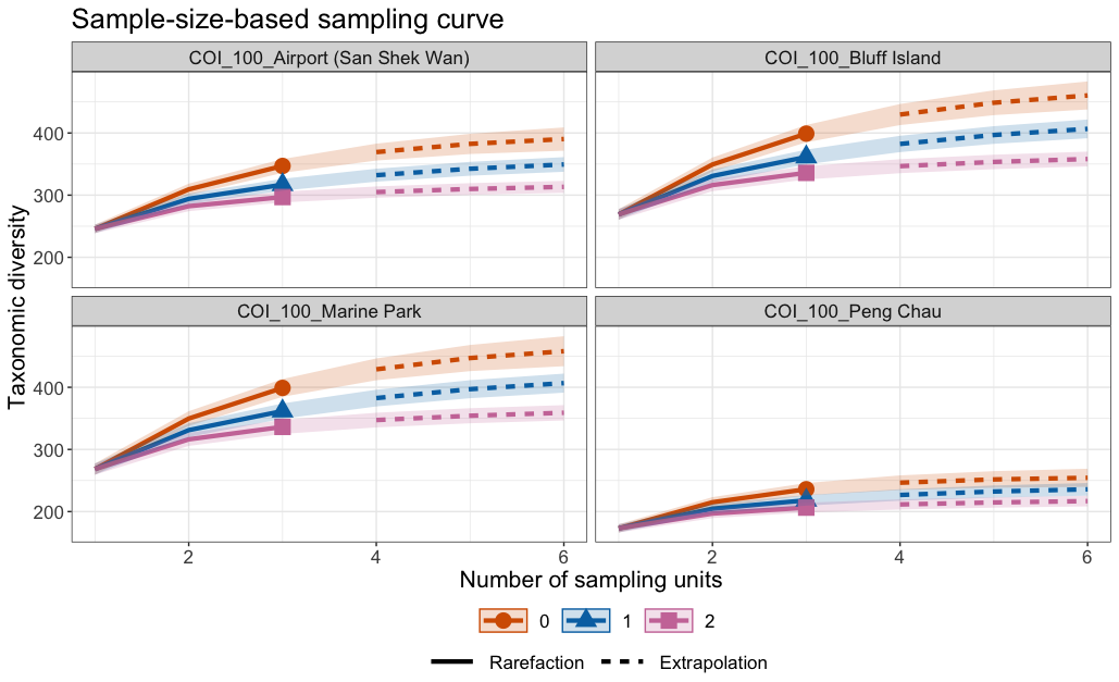
Fig. 61 : Species accumulation curves per site for the 100 µm size fraction through inter- and extrapolation from the iNEXT.3D R package.#
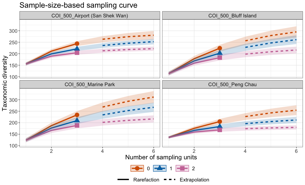
Fig. 62 : Species accumulation curves per site for the 500 µm size fraction through inter- and extrapolation from the iNEXT.3D R package.#
5.2 Alpha diversity comparison#
For the alpha diversity comparison through the Hill number framework, we can use the same data format as the species accumulation curves and use the AO3D function in the iNEXT.3D R package.
Important
Since we combined our 3 ARMS samples per site to obtain an incidence-frequency data table, we are comparing two low impacted sites against two high impacted sites. Such a comparison is not statistically sound and would require data from more low and high impacted sites. Hence, this analysis should only be seen as an introduction to the methodology, not as the outcome or endorsement of this analysis on such a data set.
# 1. run function AO3D
out.100 <- AO3D(matrix_list.100$data, diversity = 'TD', datatype = 'incidence_raw', method = 'Observed', nboot = 50, conf = 0.95)
out.500 <- AO3D(matrix_list.500$data, diversity = 'TD', datatype = 'incidence_raw', method = 'Observed', nboot = 50, conf = 0.95)
To determine differences between low and high impacted sites (and when you would have more than 2 values for each “treatment”), you can draw box plots for each Hill order and run ANOVAs to determine significant differences between the treatments for each Hill number analysed. It is important to test for the assumptions of parametric tests, such as ANOVA, to determine the need to use a non-parametric alternative instead. As mentioned above, this approach is not valid with two data points for each treatment, but below is the code to show how this would work in theory.
First, we need to subset the dataframes to contain the essential information about the Hill numbers.
################
# HILL NUMBERS #
################
# 1. subset data to include essential hill numbers, 2. add a new column to the data frame containing group info
qOrders <- c(0.0, 1.0, 2.0)
group <- c('low', 'low', 'low', 'low', 'low', 'low', 'high', 'high', 'high', 'high', 'high', 'high')
out.100 <- out.100[out.100$Order.q %in% qOrders, ]
out.100$group <- group
out.500 <- out.500[out.500$Order.q %in% qOrders, ]
out.500$group <- group
Next, we can draw the box plots.
# 1. draw boxplot for 100 size fraction
ggplot(out.100, aes(x = as.character(Order.q), y = qD, fill = group, alpha = 0.5, test = interaction(group, as.character(Order.q))))+
  geom_boxplot(outlier.size = 0) +
  geom_point(position = position_jitterdodge(jitter.width = 0.1), aes(shape = group, color = group), size = 3) +
  scale_fill_manual(values = c("lightgoldenrod", "steelblue")) +
  scale_color_manual(values = c("lightgoldenrod", "steelblue")) +
  theme_bw()

# 1. draw boxplot for 500 size fraction
ggplot(out.500, aes(x = as.character(Order.q), y = qD, fill = group, alpha = 0.5, test = interaction(group, as.character(Order.q))))+
  geom_boxplot(outlier.size = 0) +
  geom_point(position = position_jitterdodge(jitter.width = 0.1), aes(shape = group, color = group), size = 3) +
  scale_fill_manual(values = c("lightgoldenrod", "steelblue")) +
  scale_color_manual(values = c("lightgoldenrod", "steelblue")) +
  theme_bw()
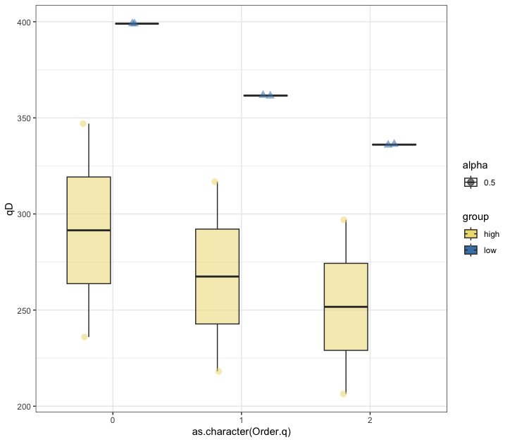
Fig. 63 : Box plot of the 100 µm size fraction of three orders of Hill numbers to compare alpha diversity measures between high and low impacted sites.#
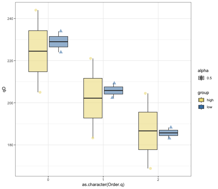
Fig. 64 : Box plot of the 500 µm size fraction of three orders of Hill numbers to compare alpha diversity measures between high and low impacted sites#
To test for significant differences between the treatments, we can run an ANOVA analysis. We will also test for the assumptions of this parametric test. Since we’re working with two groups, this ANOVA will default to a simple Student’s t-test. Note the warning before about the number of samples in the tutorial data set!
Note
The code below shows the analysis for q = 0. To test the other two orders (q = 1; q = 2), the values in the initial subsetting can be changed.
# 1. subset out.100 and out.500 to only keep q0 values
q0.100 <- out.100[out.100$Order.q %in% 0.0, ]
q0.500 <- out.500[out.500$Order.q %in% 0.0, ]

# 1. run ANOVA for q0.100
anovaHill100 <- mutate(q0.100, group = factor(group, levels = unique(group)))
Summarize(qD ~ group, data = q0.100, digits = 3)
modelq0.100 <- lm(qD ~ group, data = q0.100)
Anova(modelq0.100, type = 'II')
anova(modelq0.100)
summary(modelq0.100)

# 1. check assumptions for ANOVA q0.100
hist(residuals(modelq0.100), col = 'darkgray')
shapiro.test(residuals(modelq0.100))
plot(fitted(modelq0.100), residuals(modelq0.100))
leveneTest(qD ~ group, data = anovaHill100)
bartlett.test(qD ~ group, data = anovaHill100)

# 1. run ANOVA for q0.500
anovaHill500 <- mutate(q0.500, group = factor(group, levels = unique(group)))
Summarize(qD ~ group, data = q0.500, digits = 3)
modelq0.500 <- lm(qD ~ group, data = q0.500)
Anova(modelq0.500, type = 'II')
anova(modelq0.500)
summary(modelq0.500)

# 1. check assumptions for ANOVA q0.500
hist(residuals(modelq0.500), col = 'darkgray')
shapiro.test(residuals(modelq0.500))
plot(fitted(modelq0.500), residuals(modelq0.500))
leveneTest(qD ~ group, data = anovaHill500)
bartlett.test(qD ~ group, data = anovaHill500)
Output
> Summarize(qD ~ group, data = q0.100, digits = 3)
  group n  mean     sd min     Q1 median     Q3 max
1  high 2 291.5 78.489 236 263.75  291.5 319.25 347
2   low 2 399.0  0.000 399 399.00  399.0 399.00 399
> Anova(modelq0.100, type = 'II')
Anova Table (Type II tests)

Response: qD
           Sum Sq Df F value Pr(>F)
group     11556.3  1  3.7517 0.1924
Residuals  6160.5  2
> anova(modelq0.100)
Analysis of Variance Table

Response: qD
          Df  Sum Sq Mean Sq F value Pr(>F)
group      1 11556.3 11556.3  3.7517 0.1924
Residuals  2  6160.5  3080.2
> summary(modelq0.100)

Call:
lm(formula = qD ~ group, data = q0.100)

Residuals:
         1         12         23         34
 2.132e-14 -1.926e-14  5.550e+01 -5.550e+01

Coefficients:
            Estimate Std. Error t value Pr(>|t|)
(Intercept)   291.50      39.24   7.428   0.0176 *
grouplow      107.50      55.50   1.937   0.1924
---
Signif. codes:  0 ‘***’ 0.001 ‘**’ 0.01 ‘*’ 0.05 ‘.’ 0.1 ‘ ’ 1

Residual standard error: 55.5 on 2 degrees of freedom
Multiple R-squared:  0.6523, Adjusted R-squared:  0.4784
F-statistic: 3.752 on 1 and 2 DF,  p-value: 0.1924
> shapiro.test(residuals(modelq0.100))

 Shapiro-Wilk normality test

data:  residuals(modelq0.100)
W = 0.94466, p-value = 0.683
> leveneTest(qD ~ group, data = anovaHill100)
Levene's Test for Homogeneity of Variance (center = median)
      Df    F value    Pr(>F)
group  1 1.8254e+32 < 2.2e-16 ***
       2
---
Signif. codes:  0 ‘***’ 0.001 ‘**’ 0.01 ‘*’ 0.05 ‘.’ 0.1 ‘ ’ 1
Warning message:
In anova.lm(lm(resp ~ group)) :
  ANOVA F-tests on an essentially perfect fit are unreliable
> bartlett.test(qD ~ group, data = anovaHill100)

 Bartlett test of homogeneity of variances

data:  qD by group
Bartlett's K-squared = Inf, df = 1, p-value < 2.2e-16

Fig. 65 : Histogram to determine normal distribution of variances for the 100 µm size fraction.#
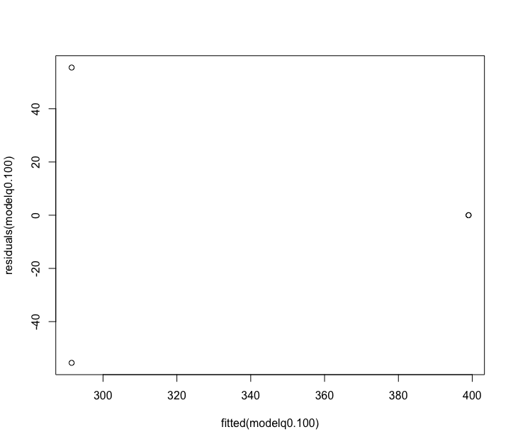
Fig. 66 : Plot of the residuals for the 100 µm size fraction.#
> Summarize(qD ~ group, data = q0.500, digits = 3)
  group n  mean     sd min     Q1 median     Q3 max
1  high 2 224.5 27.577 205 214.75  224.5 234.25 244
2   low 2 229.0  7.071 224 226.50  229.0 231.50 234
> Anova(modelq0.500, type = 'II')
Anova Table (Type II tests)

Response: qD
          Sum Sq Df F value Pr(>F)
group      20.25  1    0.05 0.8439
Residuals 810.50  2
> anova(modelq0.500)
Analysis of Variance Table

Response: qD
          Df Sum Sq Mean Sq F value Pr(>F)
group      1  20.25   20.25    0.05 0.8439
Residuals  2 810.50  405.25
> summary(modelq0.500)

Call:
lm(formula = qD ~ group, data = q0.500)

Residuals:
    1    12    23    34
  5.0  -5.0  19.5 -19.5

Coefficients:
            Estimate Std. Error t value Pr(>|t|)
(Intercept)   224.50      14.23  15.771    0.004 **
grouplow        4.50      20.13   0.224    0.844
---
Signif. codes:  0 ‘***’ 0.001 ‘**’ 0.01 ‘*’ 0.05 ‘.’ 0.1 ‘ ’ 1

Residual standard error: 20.13 on 2 degrees of freedom
Multiple R-squared:  0.02438, Adjusted R-squared:  -0.4634
F-statistic: 0.04997 on 1 and 2 DF,  p-value: 0.8439
> shapiro.test(residuals(modelq0.500))

 Shapiro-Wilk normality test

data:  residuals(modelq0.500)
W = 0.99982, p-value = 0.9995
> leveneTest(qD ~ group, data = anovaHill500)
Levene's Test for Homogeneity of Variance (center = median)
      Df    F value    Pr(>F)
group  1 2.5893e+31 < 2.2e-16 ***
       2
---
Signif. codes:  0 ‘***’ 0.001 ‘**’ 0.01 ‘*’ 0.05 ‘.’ 0.1 ‘ ’ 1
Warning message:
In anova.lm(lm(resp ~ group)) :
  ANOVA F-tests on an essentially perfect fit are unreliable
> bartlett.test(qD ~ group, data = anovaHill500)

 Bartlett test of homogeneity of variances

data:  qD by group
Bartlett's K-squared = 0.97534, df = 1, p-value = 0.3234
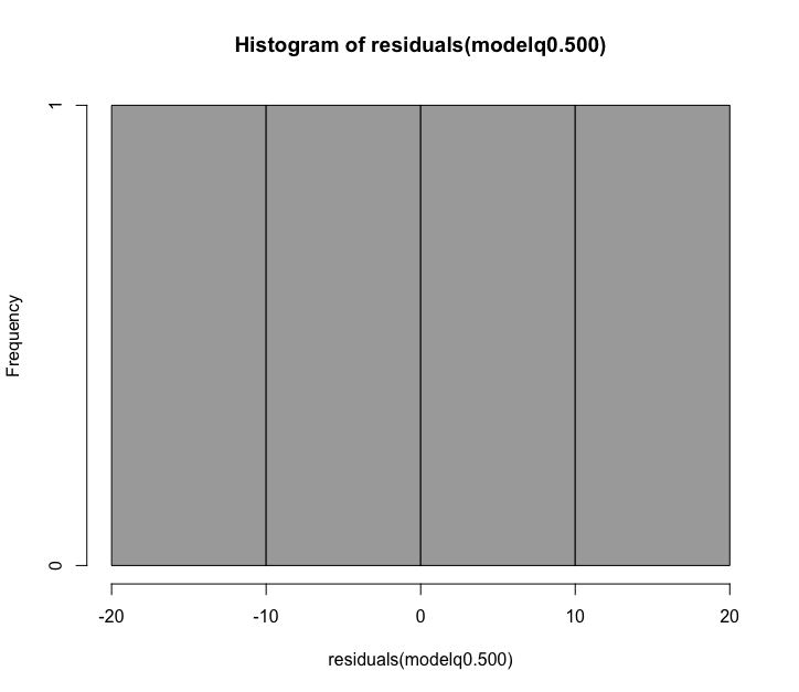
Fig. 67 : Histogram to determine normal distribution of variances for the 500 µm size fraction.#
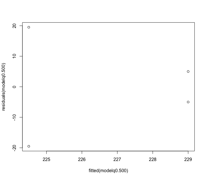
Fig. 68 : Plot of the residuals for the 500 µm size fraction.#
5.3 Estimate replication#
Through the inter- and extrapolation of alpha diversity measures calculated by the iNEXT.3D R package, we can also estimate the needed replication or sampling within a site to recover a set percentage of the diversity contained within that site. For this, we need to run the estimate3D function. We can then run a similar analysis as section 5.2 Alpha diversity comparison, whereby we can draw box plots and run ANOVAs to determine differences between treatments. The same warning applies here as mentioned in the previous section about the analysis!
########################
# ESTIMATE REPLICATION #
########################
# 1. run the estimate3D function for the 100 and 500 size fraction dataframes for q = 0
out.est.100 <- estimate3D(matrix_list.100$data, diversity = 'TD', q = 0, datatype = 'incidence_raw', base = 'coverage', level = 0.9)
out.est.500 <- estimate3D(matrix_list.500$data, diversity = 'TD', q = 0, datatype = 'incidence_raw', base = 'coverage', level = 0.9)

# 1. add a new column to the data frames containing group info
group.est <- c('low', 'low', 'high', 'high')
out.est.100$group <- group.est
out.est.500$group <- group.est

# 1. draw boxplot for size fraction 100
ggplot(out.est.100, aes(x = group, y = nt, fill = group, alpha = 0.5)) +
  geom_boxplot(outlier.size = 0, width = 0.2) +
  geom_jitter(aes(shape = group, color = group), size = 3, width = 0.1) +
  scale_fill_manual(values = c("lightgoldenrod", "steelblue")) +
  scale_color_manual(values = c("lightgoldenrod", "steelblue")) +
  theme_bw()

# 1. draw boxplot for size fraction 500
ggplot(out.est.500, aes(x = group, y = nt, fill = group, alpha = 0.5)) +
  geom_boxplot(outlier.size = 0, width = 0.2) +
  geom_jitter(aes(shape = group, color = group), size = 3, width = 0.1) +
  scale_fill_manual(values = c("lightgoldenrod", "steelblue")) +
  scale_color_manual(values = c("lightgoldenrod", "steelblue")) +
  theme_bw()
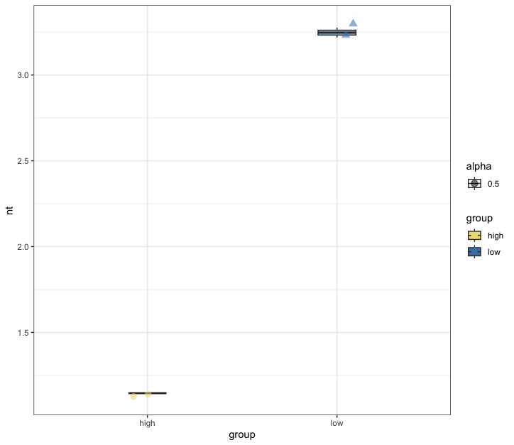
Fig. 69 : Box plot of the 100 µm size fraction of q = 0 to estimate number of samples to be collected to detect 90% of the diversity.#
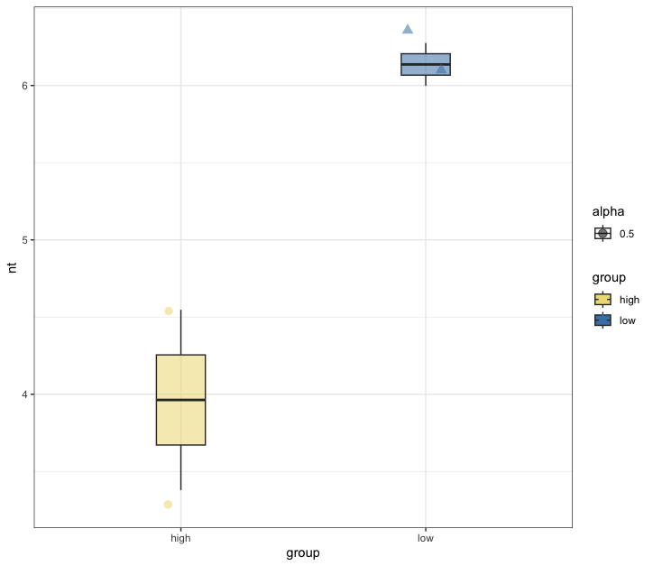
Fig. 70 : Box plot of the 500 µm size fraction of q = 0 to estimate number of samples to be collected to detect 90% of the diversity.#
# 1. run ANOVA for estimateD for 100
anovaEstimateD <- mutate(out.est.100, group = factor(group, levels = unique(group)))
Summarize(nt ~ group, data = out.est.100, digits = 3)
modelEstimateD <- lm(nt ~ group, data = out.est.100)
Anova(modelEstimateD, type = 'II')
anova(modelEstimateD)
summary(modelEstimateD)

# 1. check assumptions for ANOVA estimateD for 100
hist(residuals(modelEstimateD), col = 'darkgray')
shapiro.test(residuals(modelEstimateD))
plot(fitted(modelEstimateD), residuals(modelEstimateD))
leveneTest(nt ~ group, data = anovaEstimateD)
bartlett.test(nt ~ group, data = anovaEstimateD)
Output
> Summarize(nt ~ group, data = out.est.100, digits = 3)
  group n  mean   sd   min    Q1 median    Q3   max
1  high 2 1.146 0.00 1.146 1.146  1.146 1.146 1.146
2   low 2 3.247 0.04 3.218 3.232  3.247 3.261 3.275
> Anova(modelEstimateD, type = 'II')
Anova Table (Type II tests)

Response: nt
          Sum Sq Df F value    Pr(>F)
group     4.4129  1  5387.7 0.0001856 ***
Residuals 0.0016  2
---
Signif. codes:  0 ‘***’ 0.001 ‘**’ 0.01 ‘*’ 0.05 ‘.’ 0.1 ‘ ’ 1
> anova(modelEstimateD)
Analysis of Variance Table

Response: nt
          Df Sum Sq Mean Sq F value    Pr(>F)
group      1 4.4129  4.4129  5387.7 0.0001856 ***
Residuals  2 0.0016  0.0008
---
Signif. codes:  0 ‘***’ 0.001 ‘**’ 0.01 ‘*’ 0.05 ‘.’ 0.1 ‘ ’ 1
> summary(modelEstimateD)

Call:
lm(formula = nt ~ group, data = out.est.100)

Residuals:
         1          2          3          4
-2.862e-02  2.862e-02  3.469e-18  3.469e-18

Coefficients:
            Estimate Std. Error t value Pr(>|t|)
(Intercept)  1.14596    0.02024   56.63 0.000312 ***
grouplow     2.10068    0.02862   73.40 0.000186 ***
---
Signif. codes:  0 ‘***’ 0.001 ‘**’ 0.01 ‘*’ 0.05 ‘.’ 0.1 ‘ ’ 1

Residual standard error: 0.02862 on 2 degrees of freedom
Multiple R-squared:  0.9996, Adjusted R-squared:  0.9994
F-statistic:  5388 on 1 and 2 DF,  p-value: 0.0001856
> shapiro.test(residuals(modelEstimateD))

 Shapiro-Wilk normality test

data:  residuals(modelEstimateD)
W = 0.94466, p-value = 0.683
> leveneTest(nt ~ group, data = anovaEstimateD)
Levene's Test for Homogeneity of Variance (center = median)
      Df  F value    Pr(>F)
group  1 1.63e+28 < 2.2e-16 ***
       2
---
Signif. codes:  0 ‘***’ 0.001 ‘**’ 0.01 ‘*’ 0.05 ‘.’ 0.1 ‘ ’ 1
Warning message:
In anova.lm(lm(resp ~ group)) :
  ANOVA F-tests on an essentially perfect fit are unreliable
> bartlett.test(nt ~ group, data = anovaEstimateD)

 Bartlett test of homogeneity of variances

data:  nt by group
Bartlett's K-squared = Inf, df = 1, p-value < 2.2e-16
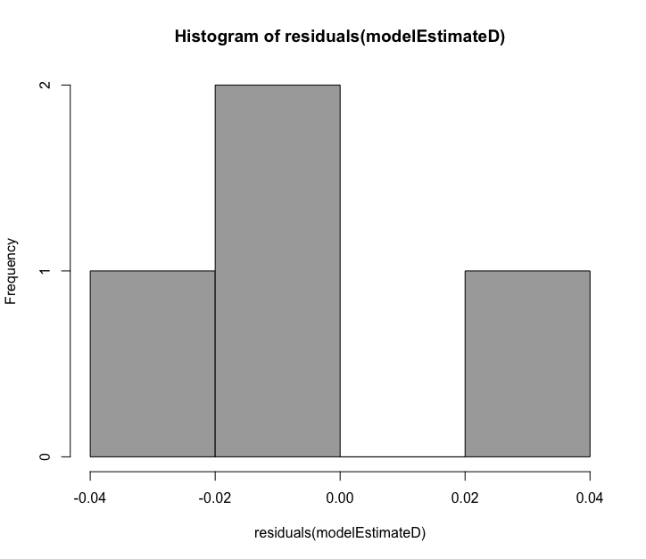
Fig. 71 : Histogram of the 100 µm size fraction of q = 0 to estimate number of samples to be collected to detect 90% of the diversity.#
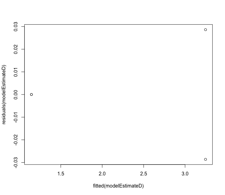
Fig. 72 : Residual plot of the 100 µm size fraction of q = 0 to estimate number of samples to be collected to detect 90% of the diversity.#
5.4 Phylodiversity#
A quick note on phylodiversity measurements: There is a push to incorporate phylogenetic relatedness in alpha diversity measurements and comparisons. Intuitively, it makes much more sense that a community comprised of 20 birds within the same family is less diverse than 20 birds comprised of different families. Such statistical frameworks that incorporate phylogenetic relatedness already exist and make use of the phylogenetic tree we generated in section Phylogenetic tree. Phylogenetic diversity measures usually take on three facets, including divergence, diversification, and survival time. Kling et al., 2018 and Alberdi & Gilbert, 2019 are two excellent publications providing additional information about this topic.
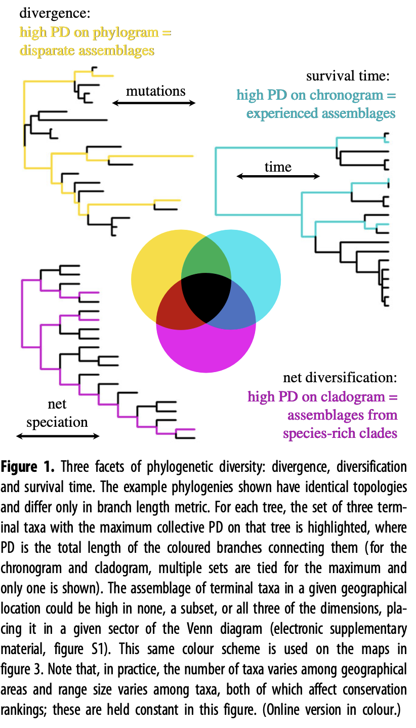
Fig. 73 : An introduction to the facets of phylogenetic diversity. Copyright: Kling et al., 2018.#
6. Beta diversity#
Besides the number of species within a site (alpha diversity), species composition or beta diversity is another important aspect of analysis within metabarcoding research. To analyse species composition between sites, we can use ordination and cluster visualisations to depict sample/site/treatment similarity or dissimilarity. PERMANOVA and PERMDISP, on the other hand, are the statistical tests to investigate significant differences between treatments based on species composition between treatments. Lastly, Indicator Species Analysis (ISA) allows us to identify which signals are driving the difference between groups.
6.1 Ordination#
Ordination is the multivariate analysis which aims to find gradients or changes in species composition across groups. Multivariate species composition can be imagined as samples in multidimensional space, where every species represents its own axis. Because multidimensional space is not easy to display, describe, or even imagine, it is worth reducing it into a few main dimensions while preserving the maximum information. In ordination space, objects that are closer together are more similar, and dissimilar objects are more separated from each other.
There are multiple ordination methods available. Some of the most common ones are Principal Components Analysis (PCA), Principle Coordinates Analysis (PCoA), and Non-metric MultiDimensional Scaling (NMDS). Although many other ordination methods exist as well, including RDA (Redundancy Analysis), CAP (Canonical Analysis of Principle coordinates), and dbRDA (Distance Cased Redundancy Analysis) The choice of ordination methods depends on (1) the type of data and (2) the similarity distance matrix you intend to use. Some methods, such as PCA are restricted to using Euclidean distance matrices, while NMDS and PCoA are able to use any distance matrix. The choice of distance matrix, is usually dependent on the type of data. For metabarcoding data, which contains lots of null values, Bray-Curtis (abundance or relative abundance) and Jaccard (presence-absence) are frequently chosen. Both these options are non-euclidean distances, which is why most metabarcoding studies opt for PCoA and NMDS ordination methods. For more information about ordination, please visit this blog or this review article.
Since metabarcoding studies usually opt for NMDS and PCoA ordination, this tutorial will cover these two options.
6.1.1 NMDS#
The first option we will cover is NMDS. NMDS is a technique that attempts to represent the pairwise dissimilarities or distances between samples in a lower-dimensional space. The goal is to position the samples in such a way that their relative distances in the ordination plot reflect the original dissimilarity structure as close as possible.
NMDS is a non-metric technique, meaning that it does not assume a linear relationship between the original distances and the distances in the ordination space. Instead, NMDS focuses on preserving the ranking or order of dissimilarities rather than their precise values.
##############
# ORDINATION #
##############
# 1. generate frequency-occurrence data frame
physeq.pa <- microbiome::transform(physeq, 'pa')
print(physeq.pa)

# 1. run NMDS
physeq.pa.nmds <- ordinate(physeq = physeq.pa, method = 'NMDS', distance = 'jaccard')

# 1. plot NMDS
sample_colors <- c("high" = "lightgoldenrod", "low" = "steelblue")
plot_ordination(physeq = physeq.pa, ordination = physeq.pa.nmds) +
  geom_point(aes(fill = SAMPLE, shape = island), size = 5) +
  stat_ellipse(aes(x = NMDS1, y = NMDS2, colour = impact), linetype = 4) +
  coord_equal() +
  scale_shape_manual(values = c(21, 22, 23, 24)) +
  scale_color_manual(values = sample_colors) +
  theme_classic() +
  theme(
    legend.text = element_text(size = 20),                               #changes legend size
    legend.title = element_blank(),                                      #removes legend title
    legend.background = element_rect(fill = "white", color = "black"))+  #adds black boarder around legend
  theme(axis.text.y.left = element_text(size = 20),
        axis.text.x = element_text(size = 20),
        axis.title.x = element_text(size = 20),
        axis.title.y = element_text(size = 20))+
  guides(fill = guide_legend(override.aes = list(shape = 21)))

# 1. output stress value
physeq.pa.nmds$stress

# 1. plot stress values in shepard's plot
stressplot(physeq.pa.nmds)
Output
> print(physeq.pa)
phyloseq-class experiment-level object
otu_table()   OTU Table:         [ 865 taxa and 24 samples ]
sample_data() Sample Data:       [ 24 samples by 32 sample variables ]
tax_table()   Taxonomy Table:    [ 865 taxa by 9 taxonomic ranks ]
refseq()      DNAStringSet:      [ 865 reference sequences ]
> physeq.pa.nmds$stress
[1] 0.08059097
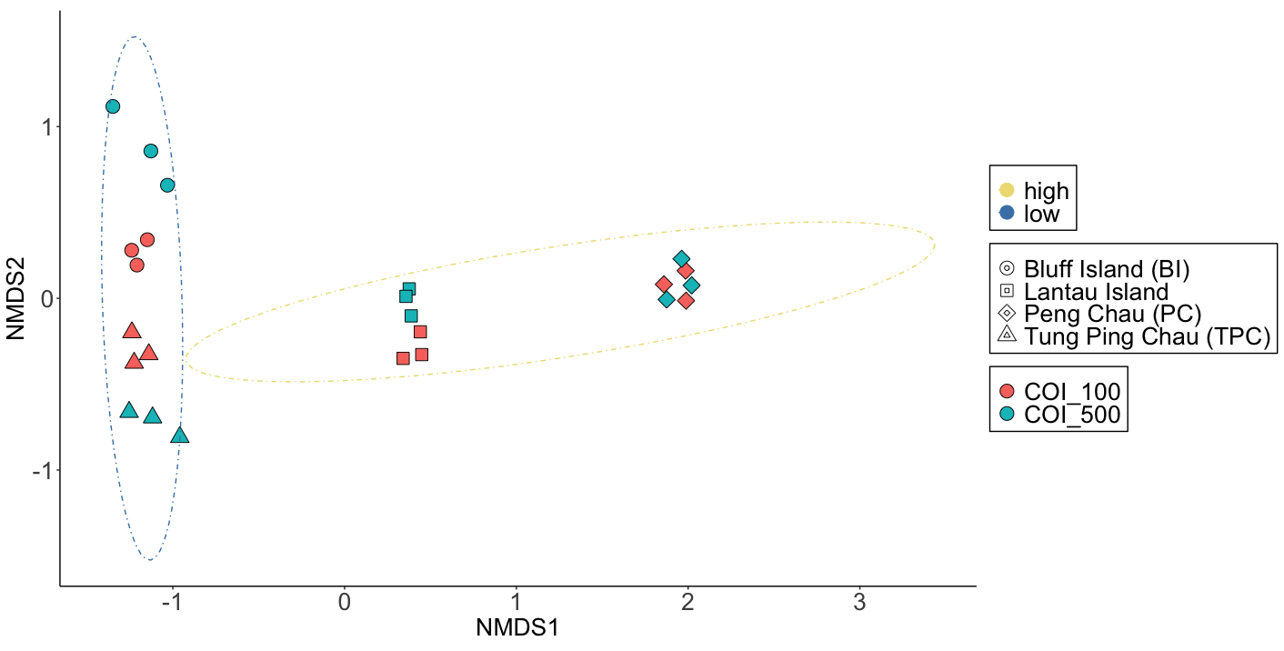
Fig. 74 : The NMDS plot whereby shapes provide information about the location, colour of shape indicate size fraction, and 95% confidence ellipses are drawn around low and high impact samples.#
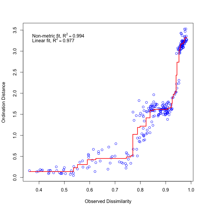
Fig. 75 : The Shepard plot of the NMDS indicating a strong correlation between observed dissimilarity and ordination distance (R2 = 0.977), highlighting an accurate representation of the NMDS.#
NMDS will provide a stress level to identify how well the NMDS plot is representing the data. As a rule of thumb, the following cut-off values are agreed upon:
stress > 0.2: poor representation; risk of false interpretation of results
0.1 < stress < 0.2: fair representation; some distances can be misleading for interpretation
0.05 < stress < 0.1: good representation; confident about the results
stress < 0.05: excellent representation.
6.1.2 PCoA#
Principal Coordinates analysis, also known as metric Multi-Dimensional Scaling (MDS), aims to preserve the original pairwise distances as closely as possible while transforming the data into a low-dimensional space. PCoA is a metric technique, thereby assuming a linear relationship between the original distances and the distances in the ordination space. If the distance measure used is Euclidean, PCoA is identical to PCA.
# 1. run PCoA
physeq.pa.pcoa <- ordinate(physeq = physeq.pa, method = 'PCoA', distance = 'jaccard')

# 1. plot PCoA
sample_colors <- c("high" = "lightgoldenrod", "low" = "steelblue")
plot_ordination(physeq = physeq.pa, ordination = physeq.pa.pcoa) +
  geom_point(aes(fill = SAMPLE, shape = island), size = 5) +
  stat_ellipse(aes(x = Axis.1, y = Axis.2, colour = impact), linetype = 4) +
  coord_equal() +
  scale_shape_manual(values = c(21, 22, 23, 24)) +
  scale_color_manual(values = sample_colors) +
  theme_classic() +
  theme(
    legend.text = element_text(size = 20),                               #changes legend size
    legend.title = element_blank(),                                      #removes legend title
    legend.background = element_rect(fill = "white", color = "black"))+  #adds black boarder around legend
  theme(axis.text.y.left = element_text(size = 20),
        axis.text.x = element_text(size = 20),
        axis.title.x = element_text(size = 20),
        axis.title.y = element_text(size = 20))+
  guides(fill = guide_legend(override.aes = list(shape = 21)))

# 1. scree plot
plot_scree(physeq.pa.pcoa)
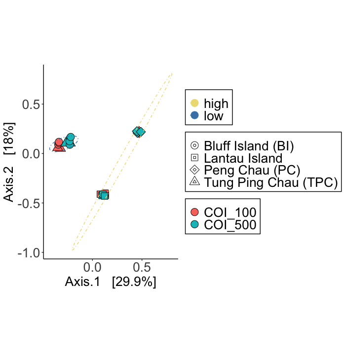
Fig. 76 : The PCoA plot whereby shapes provide information about the location, colour of shape indicate size fraction, and 95% confidence ellipses are drawn around low and high impact samples.#
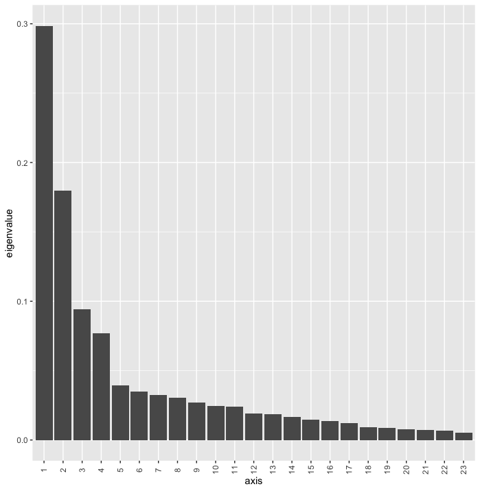
Fig. 77 : The Scree plot providing information about the percentage of variation explained on each axis.#
In PCoA, the eigenvalues represent the amount of variation explained by each axis or dimension in the ordination plot. The larger the eigenvalue, the more important that axis is in capturing the variability in the original data. We can plot a Scree plot to visualise the importance of each axis in our data set.
6.2 PERMANOVA#
While ordination is a great way to visualise differences in species community composition between samples, it does not provide a p-value to determine if those differences are significant. To check if the differences between groups are significant, we can run a PERMANOVA or PERmutational Multivariate Analysis of VAriance. The PERMANOVA procedure works by using permutation testing. Here’s a basic outline of how it works:
Data Setup: You have a dataset with multiple variables (multivariate) and multiple groups or conditions.
Dissimilarity Matrix: A dissimilarity matrix is created based on the multivariate data. This matrix quantifies the dissimilarity or distance between individual observations within the dataset (here you could pick what matrix you would like to use, in our example we are using a Jaccard matrix as we are using Presence-Absence data).
Permutation Testing: PERMANOVA works by shuffling the group labels (permuting) and then recalculating the dissimilarity matrix and relevant statistical tests. This process is repeated many times to create a distribution of test statistics under the assumption that the group labels have no effect on the data.
Comparison to Observed Data: The observed test statistic (usually a sum of squares or sums of squared distances) is then compared to the distribution of test statistics generated through permutation testing. This comparison helps determine the likelihood of observing the observed test statistic if the group labels have no effect.
P-Value Calculation: The p-value is calculated as the proportion of permuted test statistics that are more extreme than the observed test statistic. A low p-value indicates that the observed differences between groups are unlikely to occur by random chance alone.
Interpretation: If the p-value is below a pre-defined significance level (e.g., 0.05), you can then conclude that there are statistically significant differences between the groups based on the multivariate data.
#############
# PERMANOVA #
#############
# 1. extract frequency table and metadata from phyloseq object
permanova.metadata <- as(sample_data(physeq.pa), 'data.frame')
permanova.freqtable <- as.data.frame(as(otu_table(physeq.pa), 'matrix'))

# 1. create distance matrix
permanova.dist <- vegdist(t(permanova.freqtable), method = 'jaccard')
set.seed(123)
permanova.results <- adonis2(permanova.dist ~ impact, data = permanova.metadata, permutations = 10000)
permanova.results
Output
> permanova.results
Permutation test for adonis under reduced model
Terms added sequentially (first to last)
Permutation: free
Number of permutations: 10000

adonis2(formula = permanova.dist ~ impact, data = permanova.metadata, permutations = 10000)
         Df SumOfSqs      R2      F    Pr(>F)
impact    1   2.2516 0.27691 8.4251 9.999e-05 ***
Residual 22   5.8795 0.72309
Total    23   8.1311 1.00000
---
Signif. codes:  0 ‘***’ 0.001 ‘**’ 0.01 ‘*’ 0.05 ‘.’ 0.1 ‘ ’ 1
6.3 PERMDISP#
A PERMANOVA analysis can provide significant p-values if (i) the centroids of the groups are placed differently in the ordination space, (ii) the dispersion of the points between groups is different, or (iii) both. While we can verify why PERMANOVA is significant for our tutorial data, it is useful to run one additional test, PERMDISP, which provides a significant p-value only when points are dispersed differently between groups within the ordination space.
##############
# BETADISPER #
##############
mod <- betadisper(permanova.dist, permanova.metadata$impact)
mod
boxplot(mod)
permutest(mod)
Output
> permutest(mod)

Permutation test for homogeneity of multivariate dispersions
Permutation: free
Number of permutations: 999

Response: Distances
          Df   Sum Sq   Mean Sq      F N.Perm Pr(>F)
Groups     1 0.000128 0.0001278 0.0308    999  0.863
Residuals 22 0.091226 0.0041466
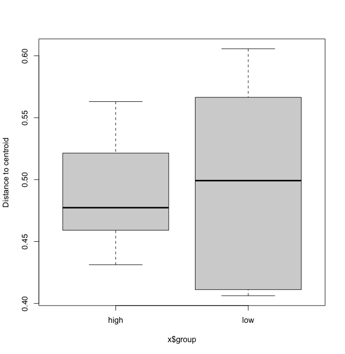
Fig. 78 : Box plot showin the distance to the centroid for each point grouped per impact variable.#
6.4 Indicator species#
To determine which signals are contributing to the difference observed in our ordination and PERMANOVA analysis, we can run an Indicator Species Analysis (ISA) using the indicspecies R package. The Indicator Value (IndVal) is a simple calculation based on the specificity (occurring only in one group or multiple) and fidelity (how frequently is it detected in each group). We can specify indvalcomp = TRUE in the summary to provide the information about the specificity (component A) and fidelity (component B). For the tutorial data, we will restrict the indicator species as the ones with perfect specificity (At=1.0) and fidelity (Bt=1.0).
#####################
# INDICATOR SPECIES #
#####################
# 1. run indicator species analysis
indval <- multipatt(t(permanova.freqtable), permanova.metadata$impact, control = how(nperm = 9999))
summary(indval, indvalcomp = TRUE, At=1.0, Bt=1.0)
Output
> summary(indval, indvalcomp = TRUE, At=1.0, Bt=1.0)

 Multilevel pattern analysis
 ---------------------------

 Association function: IndVal.g
 Significance level (alpha): 0.05
 Minimum positive predictive value (At): 1
 Minimum sensitivity (Bt): 1

 Total number of species: 865
 Selected number of species: 9
 Number of species associated to 1 group: 9

 List of species associated to each combination:

 Group high  #sps.  4
         A B stat p.value
zotu.128 1 1    1   1e-04 ***
zotu.346 1 1    1   1e-04 ***
zotu.631 1 1    1   1e-04 ***
zotu.673 1 1    1   1e-04 ***

 Group low  #sps.  5
         A B stat p.value
zotu.117 1 1    1   1e-04 ***
zotu.145 1 1    1   1e-04 ***
zotu.2   1 1    1   1e-04 ***
zotu.260 1 1    1   1e-04 ***
zotu.436 1 1    1   1e-04 ***
---
Signif. codes:  0 ‘***’ 0.001 ‘**’ 0.01 ‘*’ 0.05 ‘.’ 0.1 ‘ ’ 1
Finally, looping over the indicator species taxonomic IDs will provide information on which signals were deemed as indicative of low impact and high impact sites.
lowindval <- c('zotu.117', 'zotu.145', 'zotu.2', 'zotu.260', 'zotu.436')
highindval <- c('zotu.128', 'zotu.346', 'zotu.631', 'zotu.673')
for (item in lowindval) {
  print(taxonomyTable[item, ])
}
for (item in highindval) {
  print(taxonomyTable[item, ])
}
Output
           kingdom     phylum           class           order           family        genus          species pident qcov
zotu.117 Eukaryota Rhodophyta Florideophyceae Peyssonneliales Peyssonneliaceae Peyssonnelia Peyssonnelia_sp.  93.59   99
           kingdom     phylum   class     order     family     genus       species pident qcov
zotu.145 Eukaryota Arthropoda Insecta Blattodea Termitidae Amitermes Amitermes_sp.  75.08   98
         kingdom     phylum     class     order         family     genus               species pident qcov
zotu.2 Eukaryota Arthropoda Arachnida Opiliones Nemastomatidae Mitostoma Mitostoma_chrysomelas 76.596   89
           kingdom     phylum           class           order           family      genus        species pident qcov
zotu.260 Eukaryota Rhodophyta Florideophyceae Peyssonneliales Peyssonneliaceae Polystrata Polystrata_sp. 91.054  100
           kingdom     phylum        class    order      family    genus species pident qcov
zotu.436 Eukaryota Arthropoda Malacostraca Decapoda Galatheidae Galathea   senta    100  100
           kingdom          phylum               class           order           family         genus              species pident qcov
zotu.128 Eukaryota Bacillariophyta Coscinodiscophyceae Coscinodiscales Coscinodiscaceae Coscinodiscus Coscinodiscus_granii 88.103   99
           kingdom   phylum      class    order    family    genus       species pident qcov
zotu.346 Eukaryota Annelida Polychaeta Spionida Spionidae Polydora Polydora_aura 81.788   96
           kingdom   phylum    class        order    family  genus          species pident qcov
zotu.631 Eukaryota Cnidaria Hydrozoa Leptothecata Obeliidae Obelia Obelia_bidentata 87.622   98
           kingdom   phylum      class    order    family    genus                species pident qcov
zotu.673 Eukaryota Annelida Polychaeta Spionida Spionidae Polydora Polydora_lingshuiensis    100  100
That is it for the introduction to the statistical analysis of metabarcoding data, Congratulations on making it this far in the eDNA workshop!
